Gradients and Spheres

This example shows how you can create gradient tables and sphere objects using DIPY.

Usually, as we saw in Getting started with DIPY, you load your b-values and b-vectors from disk and then you can create your own gradient table. But this time let’s say that you are an MR physicist and you want to design a new gradient scheme or you are a scientist who wants to simulate many different gradient schemes.

Now let’s assume that you are interested in creating a multi-shell acquisition with 2-shells, one at b=1000 \(s/mm^2\) and one at b=2500 \(s/mm^2\). For both shells let’s say that we want a specific number of gradients (64) and we want to have the points on the sphere evenly distributed.

This is possible using the dipy.core.sphere.disperse_charges() which is an implementation of electrostatic repulsion Jones et al.[1] .

Let’s start by importing the necessary modules.

import numpy as np

from dipy.core.gradients import gradient_table
from dipy.core.sphere import HemiSphere, Sphere, disperse_charges
from dipy.viz import actor, window

We can first create some random points on a HemiSphere using spherical polar coordinates.

rng = np.random.default_rng()
n_pts = 64
theta = np.pi * rng.random(n_pts)
phi = 2 * np.pi * rng.random(n_pts)
hsph_initial = HemiSphere(theta=theta, phi=phi)

Next, we call dipy.core.sphere.disperse_charges() which will iteratively move the points so that the electrostatic potential energy is minimized.

hsph_updated, potential = disperse_charges(hsph_initial, 5000)

In hsph_updated we have the updated HemiSphere with the points nicely distributed on the hemisphere. Let’s visualize them.

# Enables/disables interactive visualization
interactive = False

scene = window.Scene()
scene.SetBackground(1, 1, 1)

scene.add(actor.point(hsph_initial.vertices, window.colors.red, point_radius=0.05))
scene.add(actor.point(hsph_updated.vertices, window.colors.green, point_radius=0.05))

window.record(scene=scene, out_path="initial_vs_updated.png", size=(300, 300))
if interactive:
    window.show(scene)

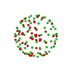
Illustration of electrostatic repulsion of red points which become green points.

We can also create a sphere from the hemisphere and show it in the following way.

sph = Sphere(xyz=np.vstack((hsph_updated.vertices, -hsph_updated.vertices)))

scene.clear()
scene.add(actor.point(sph.vertices, window.colors.green, point_radius=0.05))

window.record(scene=scene, out_path="full_sphere.png", size=(300, 300))
if interactive:
    window.show(scene)

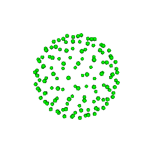
Full sphere.

It is time to create the Gradients. For this purpose we will use the function gradient_table and fill it with the hsph_updated vectors that we created above.

vertices = hsph_updated.vertices
values = np.ones(vertices.shape[0])

We need two stacks of vertices, one for every shell, and we need two sets of b-values, one at 1000 \(s/mm^2\), and one at 2500 \(s/mm^2\), as we discussed previously.

bvecs = np.vstack((vertices, vertices))
bvals = np.hstack((1000 * values, 2500 * values))

We can also add some b0s. Let’s add one at the beginning and one at the end.

bvecs = np.insert(bvecs, (0, bvecs.shape[0]), np.array([0, 0, 0]), axis=0)
bvals = np.insert(bvals, (0, bvals.shape[0]), 0)

print(bvals)
print(bvecs)

[   0. 1000. 1000. 1000. 1000. 1000. 1000. 1000. 1000. 1000. 1000. 1000.
 1000. 1000. 1000. 1000. 1000. 1000. 1000. 1000. 1000. 1000. 1000. 1000.
 1000. 1000. 1000. 1000. 1000. 1000. 1000. 1000. 1000. 1000. 1000. 1000.
 1000. 1000. 1000. 1000. 1000. 1000. 1000. 1000. 1000. 1000. 1000. 1000.
 1000. 1000. 1000. 1000. 1000. 1000. 1000. 1000. 1000. 1000. 1000. 1000.
 1000. 1000. 1000. 1000. 1000. 2500. 2500. 2500. 2500. 2500. 2500. 2500.
 2500. 2500. 2500. 2500. 2500. 2500. 2500. 2500. 2500. 2500. 2500. 2500.
 2500. 2500. 2500. 2500. 2500. 2500. 2500. 2500. 2500. 2500. 2500. 2500.
 2500. 2500. 2500. 2500. 2500. 2500. 2500. 2500. 2500. 2500. 2500. 2500.
 2500. 2500. 2500. 2500. 2500. 2500. 2500. 2500. 2500. 2500. 2500. 2500.
 2500. 2500. 2500. 2500. 2500. 2500. 2500. 2500. 2500.    0.]
[[ 0.          0.          0.        ]
 [-0.88400455 -0.27549952  0.37767178]
 [ 0.34365324  0.85415593  0.39028208]
 [-0.6134733  -0.78063201  0.11943273]
 [ 0.79805875  0.04397335  0.60097302]
 [ 0.43577355  0.89409224  0.10344312]
 [-0.39512442 -0.25433786  0.8827168 ]
 [ 0.03431186  0.9263068   0.37520449]
 [-0.69688519 -0.10042784  0.71011638]
 [-0.53419148  0.81839155  0.21183656]
 [ 0.21957237  0.04276714  0.97465837]
 [ 0.51764165  0.57803519  0.63081094]
 [ 0.46907663 -0.47560929  0.74415248]
 [-0.27126251  0.2702944   0.92377356]
 [-0.45851687  0.66081302  0.59421244]
 [-0.69041982  0.59938517  0.40504061]
 [ 0.92471155  0.34391315  0.16319405]
 [-0.98079903  0.0994493   0.16775903]
 [-0.15692523 -0.48098072  0.8625729 ]
 [ 0.62819794 -0.73260797  0.262017  ]
 [-0.74101072  0.66936578  0.05340942]
 [-0.67225545 -0.61473347  0.41252318]
 [-0.07819233  0.77250673  0.63017403]
 [-0.30110178  0.85691058  0.41838019]
 [-0.16711346 -0.02980029  0.98548721]
 [ 0.2710107  -0.88041616  0.38912799]
 [ 0.10085522 -0.74226744  0.66247059]
 [-0.69896873 -0.37365185  0.6097762 ]
 [-0.84569675 -0.50674999  0.16733636]
 [ 0.53307721  0.0549768   0.84427853]
 [-0.97938307 -0.18627262  0.07817494]
 [ 0.43441718 -0.89527432  0.09882112]
 [-0.48997984  0.05496042  0.86999949]
 [-0.28370887 -0.9409508   0.18471835]
 [ 0.66040201  0.30552289  0.68594821]
 [ 0.2459202   0.72432478  0.64410936]
 [ 0.36917282 -0.22260094  0.90230829]
 [ 0.77502261  0.62186907  0.11233346]
 [-0.4659194  -0.52332477  0.71347761]
 [-0.22303296  0.96620203  0.12926689]
 [-0.84827038  0.34971494  0.3976642 ]
 [ 0.37476523  0.35336624  0.8571367 ]
 [ 0.79371482  0.42535009  0.43484951]
 [-0.722561    0.22769721  0.6527324 ]
 [ 0.66873217 -0.22881213  0.70741946]
 [-0.08231327 -0.89456125  0.43930023]
 [ 0.11242956  0.99012508  0.08373715]
 [-0.4328074  -0.79781771  0.41971973]
 [-0.88835269  0.02034422  0.45871081]
 [ 0.11297651  0.53779361  0.83547253]
 [ 0.97879972 -0.14947035  0.14003469]
 [-0.23285111 -0.7161625   0.65794501]
 [-0.90845427  0.40610633  0.09893678]
 [ 0.93850915  0.09284575  0.33253607]
 [ 0.69897564 -0.51419647  0.49702621]
 [ 0.16980558 -0.51132963  0.84244173]
 [ 0.08176965 -0.98184724  0.17114238]
 [-0.21416803  0.55556386  0.80341823]
 [ 0.85259563 -0.48094517  0.20438307]
 [ 0.86812156 -0.24158031  0.43359417]
 [ 0.43470191 -0.70830815  0.55617786]
 [ 0.61754143  0.70522976  0.34827226]
 [-0.51970968  0.40677122  0.75129157]
 [ 0.03556459  0.27052849  0.96205483]
 [ 0.03447178 -0.24564788  0.968746  ]
 [-0.88400455 -0.27549952  0.37767178]
 [ 0.34365324  0.85415593  0.39028208]
 [-0.6134733  -0.78063201  0.11943273]
 [ 0.79805875  0.04397335  0.60097302]
 [ 0.43577355  0.89409224  0.10344312]
 [-0.39512442 -0.25433786  0.8827168 ]
 [ 0.03431186  0.9263068   0.37520449]
 [-0.69688519 -0.10042784  0.71011638]
 [-0.53419148  0.81839155  0.21183656]
 [ 0.21957237  0.04276714  0.97465837]
 [ 0.51764165  0.57803519  0.63081094]
 [ 0.46907663 -0.47560929  0.74415248]
 [-0.27126251  0.2702944   0.92377356]
 [-0.45851687  0.66081302  0.59421244]
 [-0.69041982  0.59938517  0.40504061]
 [ 0.92471155  0.34391315  0.16319405]
 [-0.98079903  0.0994493   0.16775903]
 [-0.15692523 -0.48098072  0.8625729 ]
 [ 0.62819794 -0.73260797  0.262017  ]
 [-0.74101072  0.66936578  0.05340942]
 [-0.67225545 -0.61473347  0.41252318]
 [-0.07819233  0.77250673  0.63017403]
 [-0.30110178  0.85691058  0.41838019]
 [-0.16711346 -0.02980029  0.98548721]
 [ 0.2710107  -0.88041616  0.38912799]
 [ 0.10085522 -0.74226744  0.66247059]
 [-0.69896873 -0.37365185  0.6097762 ]
 [-0.84569675 -0.50674999  0.16733636]
 [ 0.53307721  0.0549768   0.84427853]
 [-0.97938307 -0.18627262  0.07817494]
 [ 0.43441718 -0.89527432  0.09882112]
 [-0.48997984  0.05496042  0.86999949]
 [-0.28370887 -0.9409508   0.18471835]
 [ 0.66040201  0.30552289  0.68594821]
 [ 0.2459202   0.72432478  0.64410936]
 [ 0.36917282 -0.22260094  0.90230829]
 [ 0.77502261  0.62186907  0.11233346]
 [-0.4659194  -0.52332477  0.71347761]
 [-0.22303296  0.96620203  0.12926689]
 [-0.84827038  0.34971494  0.3976642 ]
 [ 0.37476523  0.35336624  0.8571367 ]
 [ 0.79371482  0.42535009  0.43484951]
 [-0.722561    0.22769721  0.6527324 ]
 [ 0.66873217 -0.22881213  0.70741946]
 [-0.08231327 -0.89456125  0.43930023]
 [ 0.11242956  0.99012508  0.08373715]
 [-0.4328074  -0.79781771  0.41971973]
 [-0.88835269  0.02034422  0.45871081]
 [ 0.11297651  0.53779361  0.83547253]
 [ 0.97879972 -0.14947035  0.14003469]
 [-0.23285111 -0.7161625   0.65794501]
 [-0.90845427  0.40610633  0.09893678]
 [ 0.93850915  0.09284575  0.33253607]
 [ 0.69897564 -0.51419647  0.49702621]
 [ 0.16980558 -0.51132963  0.84244173]
 [ 0.08176965 -0.98184724  0.17114238]
 [-0.21416803  0.55556386  0.80341823]
 [ 0.85259563 -0.48094517  0.20438307]
 [ 0.86812156 -0.24158031  0.43359417]
 [ 0.43470191 -0.70830815  0.55617786]
 [ 0.61754143  0.70522976  0.34827226]
 [-0.51970968  0.40677122  0.75129157]
 [ 0.03556459  0.27052849  0.96205483]
 [ 0.03447178 -0.24564788  0.968746  ]
 [ 0.          0.          0.        ]]

Both b-values and b-vectors look correct. Let’s now create the GradientTable.

gtab = gradient_table(bvals, bvecs=bvecs)

scene.clear()

We can also visualize the gradients. Let’s color the first shell blue and the second shell cyan.

colors_b1000 = window.colors.blue * np.ones(vertices.shape)
colors_b2500 = window.colors.cyan * np.ones(vertices.shape)
colors = np.vstack((colors_b1000, colors_b2500))
colors = np.insert(colors, (0, colors.shape[0]), np.array([0, 0, 0]), axis=0)
colors = np.ascontiguousarray(colors)

scene.add(actor.point(gtab.gradients, colors, point_radius=100))

window.record(scene=scene, out_path="gradients.png", size=(300, 300))
if interactive:
    window.show(scene)

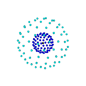
Diffusion gradients.

References

[1]

Derek K. Jones, Mark A. Horsfield, and Andrew Simmons. Optimal strategies for measuring diffusion in anisotropic systems by magnetic resonance imaging. Magnetic Resonance in Medicine, 42(3):515–25, 1999. URL: http://www.ncbi.nlm.nih.gov/pubmed/10467296, doi:10.1002/(SICI)1522-2594(199909)42:3<515::AID-MRM14>3.0.CO;2-Q.