Crossing-preserving contextual enhancement
This demo presents an example of crossing-preserving contextual enhancement of FOD/ODF fields [Meesters2016], implementing the contextual PDE framework of [Portegies2015a] for processing HARDI data. The aim is to enhance the alignment of elongated structures in the data such that crossing/junctions are maintained while reducing noise and small incoherent structures. This is achieved via a hypo-elliptic 2nd order PDE in the domain of coupled positions and orientations \(\mathbb{R}^3 \rtimes S^2\). This domain carries a non-flat geometrical differential structure that allows including a notion of alignment between neighboring points.
Let \(({\bf y},{\bf n}) \in \mathbb{R}^3\rtimes S^2\) where \({\bf y} \in \mathbb{R}^{3}\) denotes the spatial part, and \({\bf n} \in S^2\) the angular part. Let \(W:\mathbb{R}^3\rtimes S^2\times \mathbb{R}^{+} \to \mathbb{R}\) be the function representing the evolution of FOD/ODF field. Then, the contextual PDE with evolution time \(t\geq 0\) is given by:
where:
\(D^{33}>0\) is the coefficient for the spatial smoothing (which goes only in the direction of \(n\));
\(D^{44}>0\) is the coefficient for the angular smoothing (here \(\Delta_{S^2}\) denotes the Laplace-Beltrami operator on the sphere \(S^2\));
\(U:\mathbb{R}^3\rtimes S^2 \to \mathbb{R}\) is the initial condition given by the noisy FOD/ODF’s field.
This equation is solved via a shift-twist convolution (denoted by \(\ast_{\mathbb{R}^3\rtimes S^2}\)) with its corresponding kernel \(P_t:\mathbb{R}^3\rtimes S^2 \to \mathbb{R}^+\):
Here, \(R_{\bf n}\) is any 3D rotation that maps the vector \((0,0,1)\) onto \({\bf n}\).
Note that the shift-twist convolution differs from a Euclidean convolution and takes into account the non-flat structure of the space \(\mathbb{R}^3\rtimes S^2\).
The kernel \(P_t\) has a stochastic interpretation [DuitsAndFranken2011]. It can be seen as the limiting distribution obtained by accumulating random walks of particles in the position/orientation domain, where in each step the particles can (randomly) move forward/backward along their current orientation, and (randomly) change their orientation. This is an extension to the 3D case of the process for contour enhancement of 2D images.
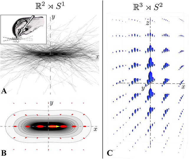
The random motion of particles (a) and its corresponding probability map (b) in 2D. The 3D kernel is shown on the right. Adapted from [Portegies2015a].
In practice, as the exact analytical formulas for the kernel \(P_t\) are unknown, we use the approximation given in [Portegies2015b].
The enhancement is evaluated on the Stanford HARDI dataset (150 orientations, b=2000 \(s/mm^2\)) where Rician noise is added. Constrained spherical deconvolution is used to model the fiber orientations.
import numpy as np
from dipy.data import fetch_stanford_hardi, read_stanford_hardi, default_sphere
from dipy.sims.voxel import add_noise

# Read data
fetch_stanford_hardi()
img, gtab = read_stanford_hardi()
data = img.get_data()

# Add Rician noise
from dipy.segment.mask import median_otsu
b0_slice = data[:, :, :, 1]
b0_mask, mask = median_otsu(b0_slice)
np.random.seed(1)
data_noisy = add_noise(data, 10.0, np.mean(b0_slice[mask]), noise_type='rician')

# Select a small part of it.
padding = 3  # Include a larger region to avoid boundary effects
data_small = data[25-padding:40+padding, 65-padding:80+padding, 35:42]
data_noisy_small = data_noisy[25-padding:40+padding,
                              65-padding:80+padding,
                              35:42]
Enables/disables interactive visualization
interactive = False
Fit an initial model to the data, in this case Constrained Spherical Deconvolution is used.
# Perform CSD on the original data
from dipy.reconst.csdeconv import auto_response
from dipy.reconst.csdeconv import ConstrainedSphericalDeconvModel
response, ratio = auto_response(gtab, data, roi_radius=10, fa_thr=0.7)
csd_model_orig = ConstrainedSphericalDeconvModel(gtab, response)
csd_fit_orig = csd_model_orig.fit(data_small)
csd_shm_orig = csd_fit_orig.shm_coeff

# Perform CSD on the original data + noise
response, ratio = auto_response(gtab, data_noisy, roi_radius=10, fa_thr=0.7)
csd_model_noisy = ConstrainedSphericalDeconvModel(gtab, response)
csd_fit_noisy = csd_model_noisy.fit(data_noisy_small)
csd_shm_noisy = csd_fit_noisy.shm_coeff
Inspired by [Rodrigues2010], a lookup-table is created, containing rotated versions of the kernel \(P_t\) sampled over a discrete set of orientations. In order to ensure rotationally invariant processing, the discrete orientations are required to be equally distributed over a sphere. By default, a sphere with 100 directions is used.
from dipy.denoise.enhancement_kernel import EnhancementKernel
from dipy.denoise.shift_twist_convolution import convolve

# Create lookup table
D33 = 1.0
D44 = 0.02
t = 1
k = EnhancementKernel(D33, D44, t)
Visualize the kernel
from dipy.viz import window, actor
from dipy.reconst.shm import sf_to_sh, sh_to_sf
ren = window.Renderer()

# convolve kernel with delta spike
spike = np.zeros((7, 7, 7, k.get_orientations().shape[0]), dtype=np.float64)
spike[3, 3, 3, 0] = 1
spike_shm_conv = convolve(sf_to_sh(spike, k.get_sphere(), sh_order=8), k,
                          sh_order=8, test_mode=True)

spike_sf_conv = sh_to_sf(spike_shm_conv, default_sphere, sh_order=8)
model_kernel = actor.odf_slicer(spike_sf_conv * 6,
                                sphere=default_sphere,
                                norm=False,
                                scale=0.4)
model_kernel.display(x=3)
ren.add(model_kernel)
ren.set_camera(position=(30, 0, 0), focal_point=(0, 0, 0), view_up=(0, 0, 1))
window.record(ren, out_path='kernel.png', size=(900, 900))
if interactive:
    window.show(ren)
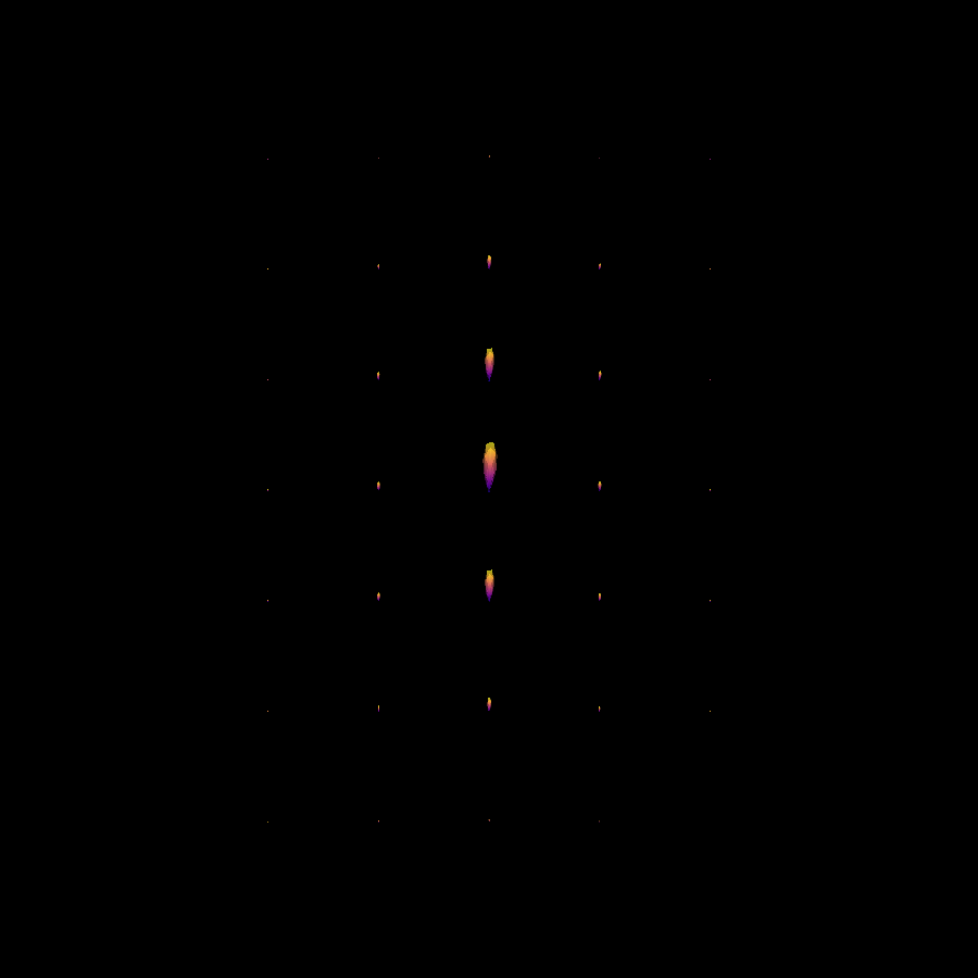
Visualization of the contour enhancement kernel.
Shift-twist convolution is applied on the noisy data
# Perform convolution
csd_shm_enh = convolve(csd_shm_noisy, k, sh_order=8)
The Sharpening Deconvolution Transform is applied to sharpen the ODF field.
# Sharpen via the Sharpening Deconvolution Transform
from dipy.reconst.csdeconv import odf_sh_to_sharp
csd_shm_enh_sharp = odf_sh_to_sharp(csd_shm_enh, default_sphere, sh_order=8,
                                    lambda_=0.1)

# Convert raw and enhanced data to discrete form
csd_sf_orig = sh_to_sf(csd_shm_orig, default_sphere, sh_order=8)
csd_sf_noisy = sh_to_sf(csd_shm_noisy, default_sphere, sh_order=8)
csd_sf_enh = sh_to_sf(csd_shm_enh, default_sphere, sh_order=8)
csd_sf_enh_sharp = sh_to_sf(csd_shm_enh_sharp, default_sphere, sh_order=8)

# Normalize the sharpened ODFs
csd_sf_enh_sharp = csd_sf_enh_sharp * np.amax(csd_sf_orig)/np.amax(csd_sf_enh_sharp) * 1.25
The end results are visualized. It can be observed that the end result after diffusion and sharpening is closer to the original noiseless dataset.
ren = window.Renderer()

# original ODF field
fodf_spheres_org = actor.odf_slicer(csd_sf_orig,
                                    sphere=default_sphere,
                                    scale=0.4,
                                    norm=False)
fodf_spheres_org.display(z=3)
fodf_spheres_org.SetPosition(0, 25, 0)
ren.add(fodf_spheres_org)

# ODF field with added noise
fodf_spheres = actor.odf_slicer(csd_sf_noisy,
                                sphere=default_sphere,
                                scale=0.4,
                                norm=False,)
fodf_spheres.SetPosition(0, 0, 0)
ren.add(fodf_spheres)

# Enhancement of noisy ODF field
fodf_spheres_enh = actor.odf_slicer(csd_sf_enh,
                                    sphere=default_sphere,
                                    scale=0.4,
                                    norm=False)
fodf_spheres_enh.SetPosition(25, 0, 0)
ren.add(fodf_spheres_enh)

# Additional sharpening
fodf_spheres_enh_sharp = actor.odf_slicer(csd_sf_enh_sharp,
                                          sphere=default_sphere,
                                          scale=0.4,
                                          norm=False)
fodf_spheres_enh_sharp.SetPosition(25, 25, 0)
ren.add(fodf_spheres_enh_sharp)

window.record(ren, out_path='enhancements.png', size=(900, 900))
if interactive:
    window.show(ren)
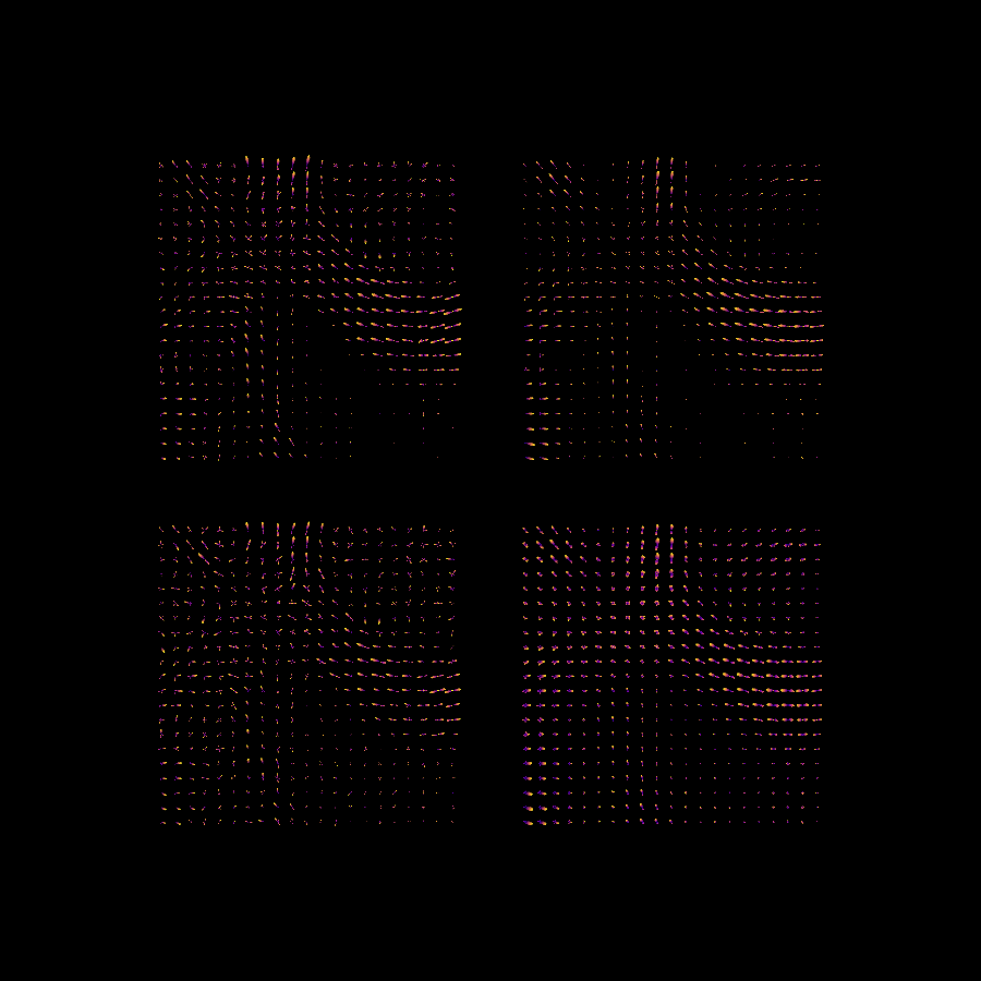
The results after enhancements. Top-left: original noiseless data. Bottom-left: original data with added Rician noise (SNR=10). Bottom-right: After enhancement of noisy data. Top-right: After enhancement and sharpening of noisy data.
References
- Meesters2016
S. Meesters, G. Sanguinetti, E. Garyfallidis, J. Portegies, R. Duits. (2016) Fast implementations of contextual PDE’s for HARDI data processing in DIPY. ISMRM 2016 conference.
- Portegies2015a(1,2)
J. Portegies, R. Fick, G. Sanguinetti, S. Meesters, G.Girard, and R. Duits. (2015) Improving Fiber Alignment in HARDI by Combining Contextual PDE flow with Constrained Spherical Deconvolution. PLoS One.
- Portegies2015b
J. Portegies, G. Sanguinetti, S. Meesters, and R. Duits. (2015) New Approximation of a Scale Space Kernel on SE(3) and Applications in Neuroimaging. Fifth International Conference on Scale Space and Variational Methods in Computer Vision.
- DuitsAndFranken2011
R. Duits and E. Franken (2011) Left-invariant diffusions on the space of positions and orientations and their application to crossing-preserving smoothing of HARDI images. International Journal of Computer Vision, 92:231-264.
- Rodrigues2010
P. Rodrigues, R. Duits, B. Romeny, A. Vilanova (2010). Accelerated Diffusion Operators for Enhancing DW-MRI. Eurographics Workshop on Visual Computing for Biology and Medicine. The Eurographics Association.
Example source code
You can download the full source code of this example. This same script is also included in the dipy source distribution under the doc/examples/ directory.