Denoise images using Local PCA via empirical thresholds
PCA-based denoising algorithms are effective denoising methods because they explore the redundancy of the multi-dimensional information of diffusion-weighted datasets. In this example, we will show how to perform the PCA-based denoising using the algorithm proposed by Manjon et al. [Manjon2013].
This algorithm involves the following steps:
First, we estimate the local noise variance at each voxel.
Then, we apply PCA in local patches around each voxel over the gradient directions.
Finally, we threshold the eigenvalues based on the local estimate of sigma and then do a PCA reconstruction
To perform PCA denoising without a prior noise standard deviation estimate please see the following example instead: denoise_mppca
Let’s load the necessary modules
import numpy as np
import nibabel as nib
import matplotlib.pyplot as plt
from time import time
from dipy.denoise.localpca import localpca
from dipy.denoise.pca_noise_estimate import pca_noise_estimate
from dipy.data import read_isbi2013_2shell
Load one of the datasets. These data were acquired with 63 gradients and 1 non-diffusion (b=0) image.
img, gtab = read_isbi2013_2shell()

data = img.get_data()
affine = img.affine

print("Input Volume", data.shape)
## Estimate the noise standard deviation
We use the pca_noise_estimate method to estimate the value of sigma to be
used in local PCA algorithm proposed by Manjon et al. [Manjon2013].
It takes both data and the gradient table object as input and returns an
estimate of local noise standard deviation as a 3D array. We return a smoothed
version, where a Gaussian filter with radius 3 voxels has been applied to the
estimate of the noise before returning it.
We correct for the bias due to Rician noise, based on an equation developed by Koay and Basser [Koay2006].
t = time()
sigma = pca_noise_estimate(data, gtab, correct_bias=True, smooth=3)
print("Sigma estimation time", time() - t)
## Perform the localPCA using the function localpca.
The localpca algorithm takes into account the multi-dimensional information of
the diffusion MR data. It performs PCA on local 4D patch and
then removes the noise components by thresholding the lowest eigenvalues.
The eigenvalue threshold will be computed from the local variance estimate
performed by the pca_noise_estimate function, if this is inputted in the
main localpca function. The relationship between the noise variance
estimate and the eigenvalue threshold can be adjusted using the input parameter
tau_factor. According to Manjon et al. [Manjon2013], this parameter is set
to 2.3.
t = time()

denoised_arr = localpca(data, sigma, tau_factor=2.3, patch_radius=2)

print("Time taken for local PCA (slow)", -t + time())
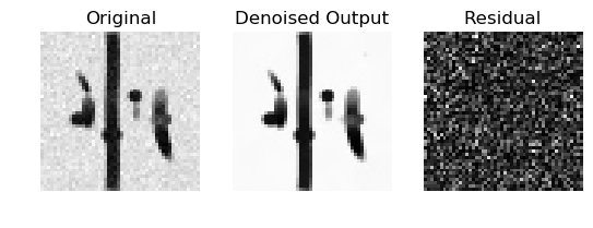
The localpca function returns the denoised data which is plotted below
(middle panel) together with the original version of the data (left panel) and
the algorithm residual (right panel) .
sli = data.shape[2] // 2
gra = data.shape[3] // 2
orig = data[:, :, sli, gra]
den = denoised_arr[:, :, sli, gra]
rms_diff = np.sqrt((orig - den) ** 2)

fig, ax = plt.subplots(1, 3)
ax[0].imshow(orig, cmap='gray', origin='lower', interpolation='none')
ax[0].set_title('Original')
ax[0].set_axis_off()
ax[1].imshow(den, cmap='gray', origin='lower', interpolation='none')
ax[1].set_title('Denoised Output')
ax[1].set_axis_off()
ax[2].imshow(rms_diff, cmap='gray', origin='lower', interpolation='none')
ax[2].set_title('Residual')
ax[2].set_axis_off()
plt.savefig('denoised_localpca.png', bbox_inches='tight')

print("The result saved in denoised_localpca.png")

Below we show how the denoised data can be saved.
nib.save(nib.Nifti1Image(denoised_arr,
                         affine), 'denoised_localpca.nii.gz')

print("Entire denoised data saved in denoised_localpca.nii.gz")
- Manjon2013(1,2,3)
Manjon JV, Coupe P, Concha L, Buades A, Collins DL “Diffusion Weighted Image Denoising Using Overcomplete Local PCA” (2013). PLoS ONE 8(9): e73021. doi:10.1371/journal.pone.0073021.
- Koay2006
Koay CG, Basser PJ (2006). “Analytically exact correction scheme for signal extraction from noisy magnitude MR signals”. JMR 179: 317-322.
Example source code
You can download the full source code of this example. This same script is also included in the dipy source distribution under the doc/examples/ directory.
