
Crossing invariant fiber response function with FORECAST model
We show how to obtain a voxel specific response function in the form of axially symmetric tensor and the fODF using the FORECAST model from [Anderson2005] , [Kaden2016] and [Zucchelli2017].
First import the necessary modules:
import matplotlib.pyplot as plt
from dipy.reconst.forecast import ForecastModel
from dipy.viz import actor, window
from dipy.data import fetch_cenir_multib, read_cenir_multib, get_sphere
Download and read the data for this tutorial. Our implementation of FORECAST requires multi-shell data. fetch_cenir_multib() provides data acquired using the shells at b-values 1000, 2000, and 3000 (see MAPMRI example for more information on this dataset).
fetch_cenir_multib(with_raw=False)

bvals = [1000, 2000, 3000]
img, gtab = read_cenir_multib(bvals)
data = img.get_data()
Let us consider only a single slice for the FORECAST fitting
data_small = data[18:87, 51:52, 10:70]
mask_small = data_small[..., 0] > 1000
Instantiate the FORECAST Model.
“sh_order” is the spherical harmonics order used for the fODF.
dec_alg is the spherical deconvolution algorithm used for the FORECAST basis fitting, in this case we used the Constrained Spherical Deconvolution (CSD) algorithm.
fm = ForecastModel(gtab, sh_order=6, dec_alg='CSD')
Fit the FORECAST to the data
f_fit = fm.fit(data_small, mask_small)
Calculate the crossing invariant tensor indices [Kaden2016] : the parallel diffusivity, the perpendicular diffusivity, the fractional anisotropy and the mean diffusivity.
d_par = f_fit.dpar
d_perp = f_fit.dperp
fa = f_fit.fractional_anisotropy()
md = f_fit.mean_diffusivity()
Show the indices and save them in FORECAST_indices.png.
fig = plt.figure(figsize=(6, 6))
ax1 = fig.add_subplot(2, 2, 1, title='parallel diffusivity')
ax1.set_axis_off()
ind = ax1.imshow(d_par[:, 0, :].T, interpolation='nearest',
                 origin='lower', cmap=plt.cm.gray)
plt.colorbar(ind, shrink=0.6)
ax2 = fig.add_subplot(2, 2, 2, title='perpendicular diffusivity')
ax2.set_axis_off()
ind = ax2.imshow(d_perp[:, 0, :].T, interpolation='nearest',
                 origin='lower', cmap=plt.cm.gray)
plt.colorbar(ind, shrink=0.6)
ax3 = fig.add_subplot(2, 2, 3, title='fractional anisotropy')
ax3.set_axis_off()
ind = ax3.imshow(fa[:, 0, :].T, interpolation='nearest',
                 origin='lower', cmap=plt.cm.gray)
plt.colorbar(ind, shrink=0.6)
ax4 = fig.add_subplot(2, 2, 4, title='mean diffusivity')
ax4.set_axis_off()
ind = ax4.imshow(md[:, 0, :].T, interpolation='nearest',
                 origin='lower', cmap=plt.cm.gray)
plt.colorbar(ind, shrink=0.6)
plt.savefig('FORECAST_indices.png', dpi=300, bbox_inches='tight')
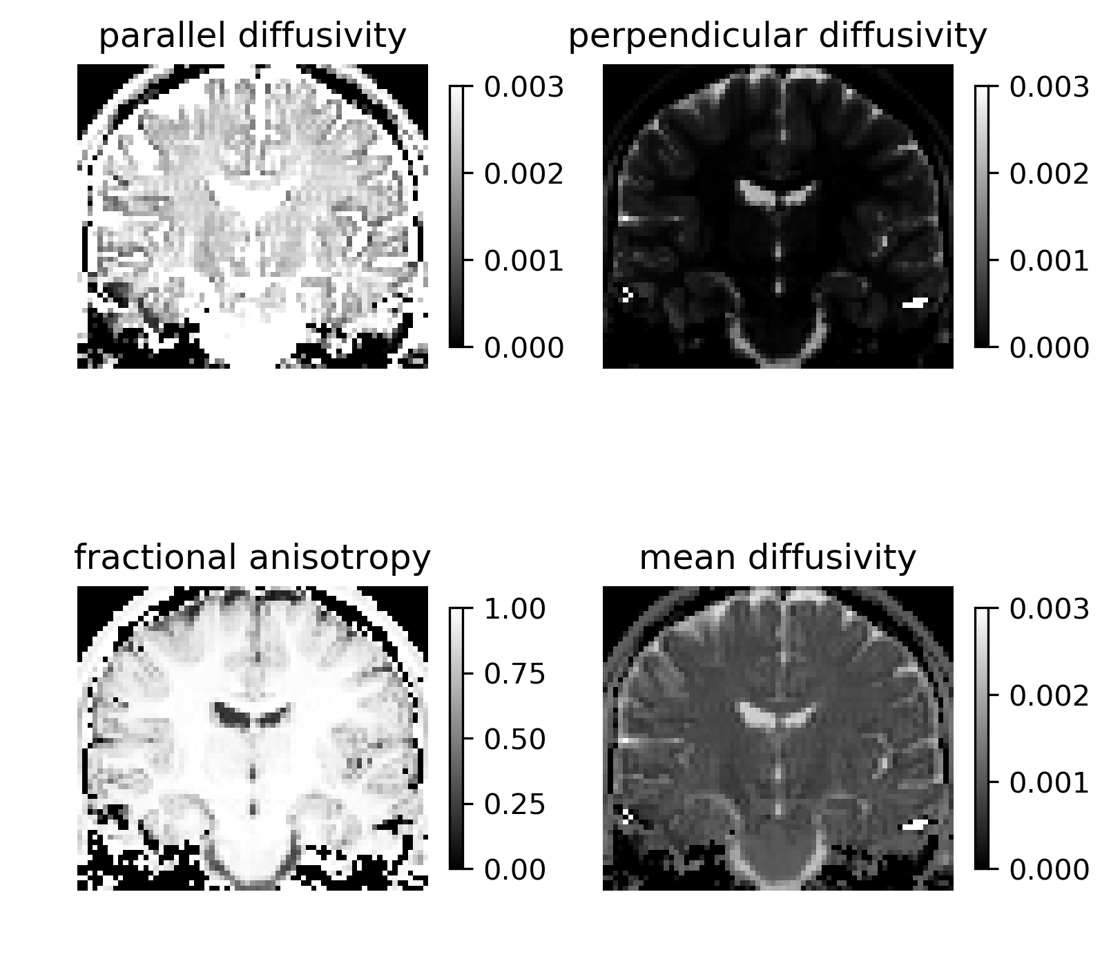
FORECAST scalar indices.
Load an ODF reconstruction sphere
sphere = get_sphere('repulsion724')
Compute the fODFs.
odf = f_fit.odf(sphere)
print('fODF.shape (%d, %d, %d, %d)' % odf.shape)
Display a part of the fODFs
odf_actor = actor.odf_slicer(odf[16:36, :, 30:45], sphere=sphere,
                             colormap='plasma', scale=0.6)
odf_actor.display(y=0)
odf_actor.RotateX(-90)
ren = window.Renderer()
ren.add(odf_actor)
window.record(ren, out_path='fODFs.png', size=(600, 600), magnification=4)
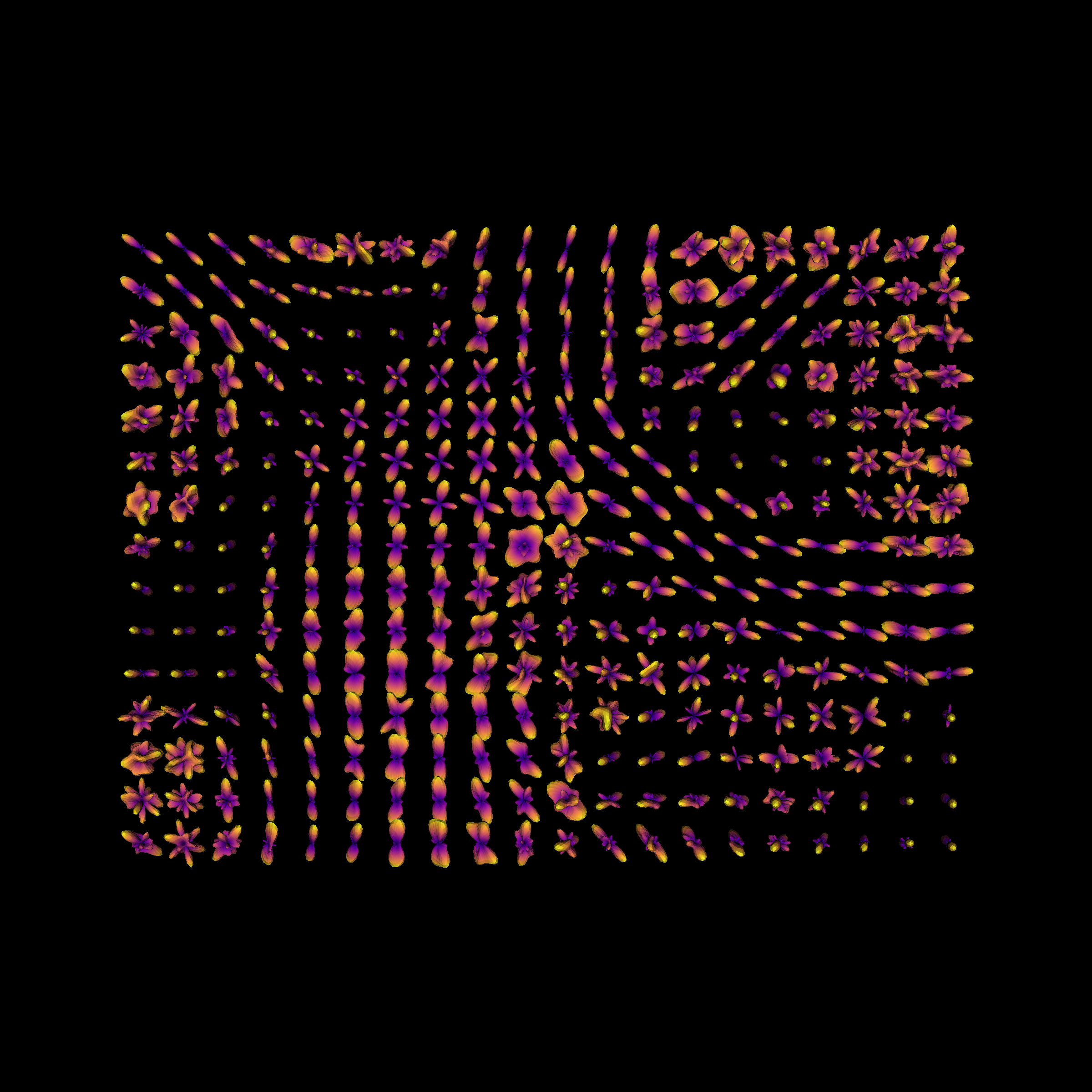
Fiber Orientation Distribution Functions, in a small ROI of the brain.
References
- Anderson2005
Anderson A. W., “Measurement of Fiber Orientation Distributions Using High Angular Resolution Diffusion Imaging”, Magnetic Resonance in Medicine, 2005.
- Kaden2016(1,2)
Kaden E. et al., “Quantitative Mapping of the Per-Axon Diffusion Coefficients in Brain White Matter”, Magnetic Resonance in Medicine, 2016.
- Zucchelli2017
Zucchelli E. et al., “A generalized SMT-based framework for Diffusion MRI microstructural model estimation”, MICCAI Workshop on Computational DIFFUSION MRI (CDMRI), 2017.
Example source code
You can download the full source code of this example. This same script is also included in the dipy source distribution under the doc/examples/ directory.