Introduction to Basic Tracking
Local fiber tracking is an approach used to model white matter fibers by creating streamlines from local directional information. The idea is as follows: if the local directionality of a tract/pathway segment is known, one can integrate along those directions to build a complete representation of that structure. Local fiber tracking is widely used in the field of diffusion MRI because it is simple and robust.
In order to perform local fiber tracking, three things are needed: 1) A method for getting directions from a diffusion data set. 2) A method for identifying when the tracking must stop. 3) A set of seeds from which to begin tracking. This example shows how to combine the 3 parts described above to create a tractography reconstruction from a diffusion data set.
To begin, let’s load an example HARDI data set from Stanford. If you have not already downloaded this data set, the first time you run this example you will need to be connected to the internet and this dataset will be downloaded to your computer.
# Enables/disables interactive visualization
interactive = False

from dipy.data import read_stanford_labels

hardi_img, gtab, labels_img = read_stanford_labels()
data = hardi_img.get_data()
labels = labels_img.get_data()
affine = hardi_img.affine
This dataset provides a label map in which all white matter tissues are labeled either 1 or 2. Lets create a white matter mask to restrict tracking to the white matter.
white_matter = (labels == 1) | (labels == 2)
1. The first thing we need to begin fiber tracking is a way of getting
directions from this diffusion data set. In order to do that, we can fit the
data to a Constant Solid Angle ODF Model. This model will estimate the
Orientation Distribution Function (ODF) at each voxel. The ODF is the
distribution of water diffusion as a function of direction. The peaks of an ODF
are good estimates for the orientation of tract segments at a point in the
image. Here, we use peaks_from_model to fit the data and calculated the
fiber directions in all voxels of the white matter.
from dipy.reconst.csdeconv import auto_response
from dipy.reconst.shm import CsaOdfModel
from dipy.data import default_sphere
from dipy.direction import peaks_from_model

response, ratio = auto_response(gtab, data, roi_radius=10, fa_thr=0.7)
csa_model = CsaOdfModel(gtab, sh_order=6)
csa_peaks = peaks_from_model(csa_model, data, default_sphere,
                             relative_peak_threshold=.8,
                             min_separation_angle=45,
                             mask=white_matter)
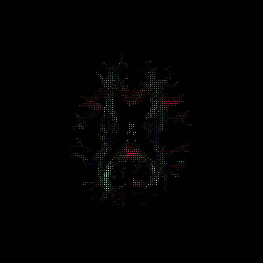
For quality assurance we can also visualize a slice from the direction field
which we will use as the basis to perform the tracking. The visualization will
be done using the fury python package
from dipy.viz import window, actor, has_fury

if has_fury:
    ren = window.Renderer()
    ren.add(actor.peak_slicer(csa_peaks.peak_dirs,
                              csa_peaks.peak_values,
                              colors=None))

    window.record(ren, out_path='csa_direction_field.png', size=(900, 900))

    if interactive:
        window.show(ren, size=(800, 800))

Direction Field (peaks)
2. Next we need some way of restricting the fiber tracking to areas with good directionality information. We’ve already created the white matter mask, but we can go a step further and restrict fiber tracking to those areas where the ODF shows significant restricted diffusion by thresholding on the generalized fractional anisotropy (GFA).
from dipy.tracking.stopping_criterion import ThresholdStoppingCriterion

stopping_criterion = ThresholdStoppingCriterion(csa_peaks.gfa, .25)
Again, for quality assurance we can also visualize a slice the GFA and the resulting tracking mask.
import matplotlib.pyplot as plt

sli = csa_peaks.gfa.shape[2] // 2
plt.figure('GFA')
plt.subplot(1, 2, 1).set_axis_off()
plt.imshow(csa_peaks.gfa[:, :, sli].T, cmap='gray', origin='lower')

plt.subplot(1, 2, 2).set_axis_off()
plt.imshow((csa_peaks.gfa[:, :, sli] > 0.25).T, cmap='gray', origin='lower')

plt.savefig('gfa_tracking_mask.png')
An example of tracking mask derived from the generalized fractional anisotropy (GFA).
3. Before we can begin tracking is to specify where to “seed” (begin) the fiber
tracking. Generally, the seeds chosen will depend on the pathways one is
interested in modeling. In this example, we’ll use a \(2 \times 2 \times 2\) grid
of seeds per voxel, in a sagittal slice of the corpus callosum. Tracking from
this region will give us a model of the corpus callosum tract. This slice has
label value 2 in the labels image.
from dipy.tracking import utils

seed_mask = (labels == 2)
seeds = utils.seeds_from_mask(seed_mask, affine, density=[2, 2, 2])
Finally, we can bring it all together using LocalTracking, performing Using
the EuDX algorithm [Garyfallidis12]. EuDX [Garyfallidis12] is a fast
algorithm that we use here to generate streamlines. This algorithm is what is
used here and the default option when providing the output of peaks directly
in LocalTracking.
from dipy.tracking.local_tracking import LocalTracking
from dipy.tracking.streamline import Streamlines

# Initialization of LocalTracking. The computation happens in the next step.
streamlines_generator = LocalTracking(csa_peaks, stopping_criterion, seeds,
                                      affine=affine, step_size=.5)
# Generate streamlines object
streamlines = Streamlines(streamlines_generator)
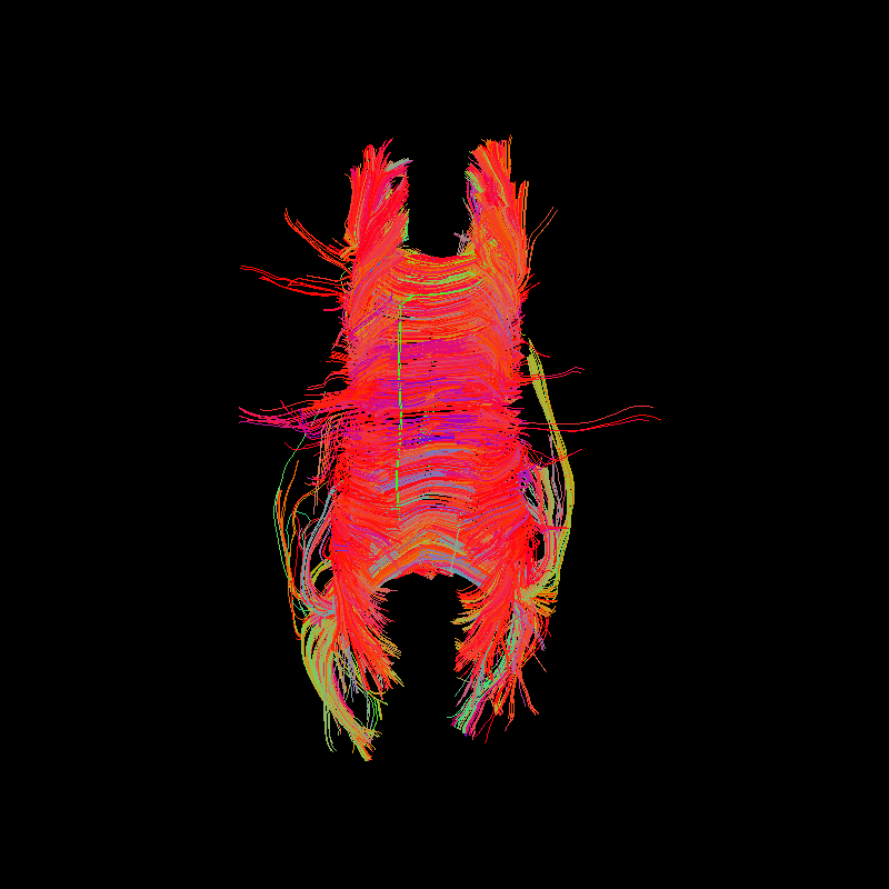
We will then display the resulting streamlines using the fury
python package.
from dipy.viz import colormap

if has_fury:
    # Prepare the display objects.
    color = colormap.line_colors(streamlines)

    streamlines_actor = actor.line(streamlines,
                                   colormap.line_colors(streamlines))

    # Create the 3D display.
    r = window.Renderer()
    r.add(streamlines_actor)

    # Save still images for this static example. Or for interactivity use
    window.record(r, out_path='tractogram_EuDX.png', size=(800, 800))
    if interactive:
        window.show(r)

Corpus Callosum using EuDx
We’ve created a deterministic set of streamlines using the EuDX algorithm. This is so called deterministic because if you repeat the fiber tracking (keeping all the inputs the same) you will get exactly the same set of streamlines. We can save the streamlines as a Trackvis file so it can be loaded into other software for visualization or further analysis.
from dipy.io.stateful_tractogram import Space, StatefulTractogram
from dipy.io.streamline import save_trk

sft = StatefulTractogram(streamlines, hardi_img, Space.RASMM)
save_trk(sft, "tractogram_EuDX.trk", streamlines)
References
PhD thesis, University of Cambridge, 2012.
Example source code
You can download the full source code of this example. This same script is also included in the dipy source distribution under the doc/examples/ directory.
