Reconstruction of the diffusion signal with the kurtosis tensor model
The diffusion kurtosis model is an expansion of the diffusion tensor model (see Reconstruction of the diffusion signal with the Tensor model). In addition to the diffusion tensor (DT), the diffusion kurtosis model quantifies the degree to which water diffusion in biological tissues is non-Gaussian using the kurtosis tensor (KT) [Jensen2005].
Measurements of non-Gaussian diffusion from the diffusion kurtosis model are of interest because they can be used to charaterize tissue microstructural heterogeneity [Jensen2010]. Moreover, DKI can be used to: 1) derive concrete biophysical parameters, such as the density of axonal fibers and diffusion tortuosity [Fierem2011] (see Reconstruction of the diffusion signal with the WMTI model); and 2) resolve crossing fibers in tractography and to obtain invariant rotational measures not limited to well-aligned fiber populations [NetoHe2015].
The diffusion kurtosis model expresses the diffusion-weighted signal as:
where \(\mathbf{b}\) is the applied diffusion weighting (which is dependent on the measurement parameters), \(S_0\) is the signal in the absence of diffusion gradient sensitization, \(\mathbf{D(n)}\) is the value of diffusion along direction \(\mathbf{n}\), and \(\mathbf{K(n)}\) is the value of kurtosis along direction \(\mathbf{n}\). The directional diffusion \(\mathbf{D(n)}\) and kurtosis \(\mathbf{K(n)}\) can be related to the diffusion tensor (DT) and kurtosis tensor (KT) using the following equations:
and
where \(D_{ij}\) are the elements of the second-order DT, and \(W_{ijkl}\) the elements of the fourth-order KT and \(MD\) is the mean diffusivity. As the DT, KT has antipodal symmetry and thus only 15 Wijkl elemments are needed to fully characterize the KT:
In the following example we show how to fit the diffusion kurtosis model on diffusion-weighted multi-shell datasets and how to estimate diffusion kurtosis based statistics.
First, we import all relevant modules:
import numpy as np
import matplotlib.pyplot as plt
import dipy.reconst.dki as dki
import dipy.reconst.dti as dti
from dipy.data import fetch_cfin_multib
from dipy.data import read_cfin_dwi
from dipy.segment.mask import median_otsu
from scipy.ndimage.filters import gaussian_filter
DKI requires multi-shell data, i.e. data acquired from more than one non-zero b-value. Here, we use fetch to download a multi-shell dataset which was kindly provided by Hansen and Jespersen (more details about the data are provided in their paper [Hansen2016]). The total size of the downloaded data is 192 MBytes, however you only need to fetch it once.
fetch_cfin_multib()

img, gtab = read_cfin_dwi()

data = img.get_data()

affine = img.affine
Function read_cfin_multib return img and gtab which contains respectively
a nibabel Nifti1Image object (where the data can be extracted) and a
GradientTable object with information about the b-values and b-vectors.
Before fitting the data, we preform some data pre-processing. We first compute a brain mask to avoid unnecessary calculations on the background of the image.
maskdata, mask = median_otsu(data, vol_idx=[0, 1], median_radius=4, numpass=2,
                             autocrop=False, dilate=1)
Since the diffusion kurtosis models involves the estimation of a large number of parameters [TaxCMW2015] and since the non-Gaussian components of the diffusion signal are more sensitive to artefacts [NetoHe2012], it might be favorable to suppress the effects of noise and artefacts before diffusion kurtosis fitting. In this example the effects of noise and artefacts are suppress by using 3D Gaussian smoothing (with a Gaussian kernel with fwhm=1.25) as suggested by pioneer DKI studies (e.g. [Jensen2005], [NetoHe2012]). Although here the Gaussian smoothing is used so that results are comparable to these studies, it is important to note that more advanced noise and artifact suppression algorithms are available in DIPY (e.g. the non-local means filter example-denoise-nlmeans).
fwhm = 1.25
gauss_std = fwhm / np.sqrt(8 * np.log(2))  # converting fwhm to Gaussian std
data_smooth = np.zeros(data.shape)
for v in range(data.shape[-1]):
    data_smooth[..., v] = gaussian_filter(data[..., v], sigma=gauss_std)
Now that we have loaded and pre-processed the data we can go forward with DKI fitting. For this, the DKI model is first defined for the data’s GradientTable object by instantiating the DiffusionKurtosisModel object in the following way:
dkimodel = dki.DiffusionKurtosisModel(gtab)
To fit the data using the defined model object, we call the fit function of
this object:
dkifit = dkimodel.fit(data_smooth, mask=mask)
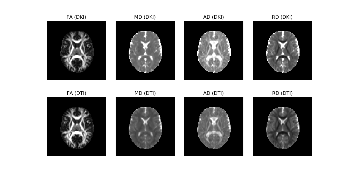
The fit method creates a DiffusionKurtosisFit object, which contains all the diffusion and kurtosis fitting parameters and other DKI attributes. For instance, since the diffusion kurtosis model estimates the diffusion tensor, all diffusion standard tensor statistics can be computed from the DiffusionKurtosisFit instance. For example, we show below how to extract the fractional anisotropy (FA), the mean diffusivity (MD), the axial diffusivity (AD) and the radial diffusivity (RD) from the DiffusionKurtosisiFit instance.
FA = dkifit.fa
MD = dkifit.md
AD = dkifit.ad
RD = dkifit.rd
Note that these four standard measures could also be computed from DIPY’s DTI
module. Theoretically, computing these measures from both models should be
analogous. However, according to recent studies, the diffusion statistics from
the kurtosis model are expected to have better accuracy [Veraar2011],
[NetoHe2012]. For comparison purposes, we calculate below the FA, MD, AD, and
RD using DIPY’s TensorModel.
tenmodel = dti.TensorModel(gtab)
tenfit = tenmodel.fit(data_smooth, mask=mask)

dti_FA = tenfit.fa
dti_MD = tenfit.md
dti_AD = tenfit.ad
dti_RD = tenfit.rd
The DT based measures can be easily visualized using matplotlib. For example, the FA, MD, AD, and RD obtained from the diffusion kurtosis model (upper panels) and the tensor model (lower panels) are plotted for a selected axial slice.
axial_slice = 9

fig1, ax = plt.subplots(2, 4, figsize=(12, 6),
                        subplot_kw={'xticks': [], 'yticks': []})

fig1.subplots_adjust(hspace=0.3, wspace=0.05)

ax.flat[0].imshow(FA[:, :, axial_slice].T, cmap='gray',
                  vmin=0, vmax=0.7, origin='lower')
ax.flat[0].set_title('FA (DKI)')
ax.flat[1].imshow(MD[:, :, axial_slice].T, cmap='gray',
                  vmin=0, vmax=2.0e-3, origin='lower')
ax.flat[1].set_title('MD (DKI)')
ax.flat[2].imshow(AD[:, :, axial_slice].T, cmap='gray',
                  vmin=0, vmax=2.0e-3, origin='lower')
ax.flat[2].set_title('AD (DKI)')
ax.flat[3].imshow(RD[:, :, axial_slice].T, cmap='gray',
                  vmin=0, vmax=2.0e-3, origin='lower')
ax.flat[3].set_title('RD (DKI)')

ax.flat[4].imshow(dti_FA[:, :, axial_slice].T, cmap='gray',
                  vmin=0, vmax=0.7, origin='lower')
ax.flat[4].set_title('FA (DTI)')
ax.flat[5].imshow(dti_MD[:, :, axial_slice].T, cmap='gray',
                  vmin=0, vmax=2.0e-3, origin='lower')
ax.flat[5].set_title('MD (DTI)')
ax.flat[6].imshow(dti_AD[:, :, axial_slice].T, cmap='gray',
                  vmin=0, vmax=2.0e-3, origin='lower')
ax.flat[6].set_title('AD (DTI)')
ax.flat[7].imshow(dti_RD[:, :, axial_slice].T, cmap='gray',
                  vmin=0, vmax=2.0e-3, origin='lower')
ax.flat[7].set_title('RD (DTI)')

plt.show()
fig1.savefig('Diffusion_tensor_measures_from_DTI_and_DKI.png')

Diffusion tensor measures obtained from the diffusion tensor estimated from DKI (upper panels) and DTI (lower panels).
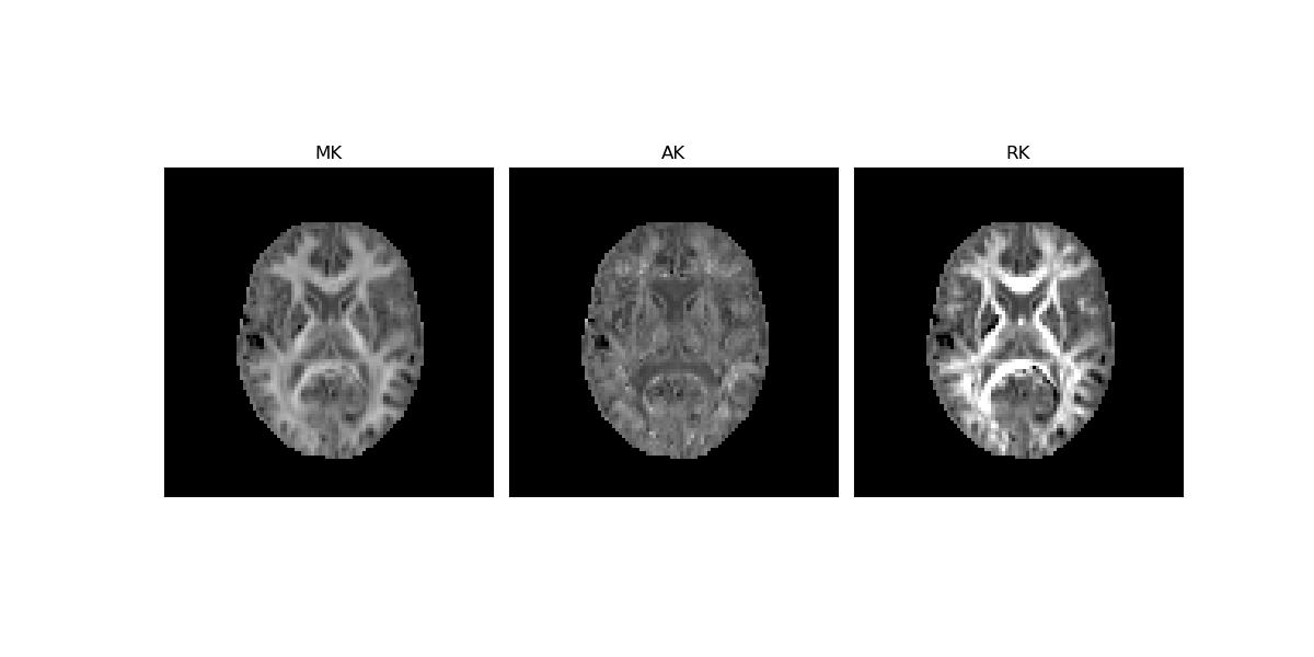
In addition to the standard diffusion statistics, the DiffusionKurtosisFit instance can be used to estimate the non-Gaussian measures of mean kurtosis (MK), the axial kurtosis (AK) and the radial kurtosis (RK).
Kurtosis measures are susceptible to high amplitude outliers. The impact of high amplitude kurtosis outliers can be removed by introducing as an optional input the extremes of the typical values of kurtosis. Here these are assumed to be on the range between 0 and 3):
MK = dkifit.mk(0, 3)
AK = dkifit.ak(0, 3)
RK = dkifit.rk(0, 3)
Now we are ready to plot the kurtosis standard measures using matplotlib:
fig2, ax = plt.subplots(1, 3, figsize=(12, 6),
                        subplot_kw={'xticks': [], 'yticks': []})

fig2.subplots_adjust(hspace=0.3, wspace=0.05)

ax.flat[0].imshow(MK[:, :, axial_slice].T, cmap='gray', vmin=0, vmax=1.5,
                  origin='lower')
ax.flat[0].set_title('MK')
ax.flat[1].imshow(AK[:, :, axial_slice].T, cmap='gray', vmin=0, vmax=1.5,
                  origin='lower')
ax.flat[1].set_title('AK')
ax.flat[2].imshow(RK[:, :, axial_slice].T, cmap='gray', vmin=0, vmax=1.5,
                  origin='lower')
ax.flat[2].set_title('RK')

plt.show()
fig2.savefig('Kurtosis_tensor_standard_measures.png')

Kurtosis tensor standard measures obtained from the kurtosis tensor.
The non-Gaussian behaviour of the diffusion signal is larger when water diffusion is restricted by compartments and barriers (e.g., myelin sheath). Therefore, as the figure above shows, white matter kurtosis values are smaller along the axial direction of fibers (smaller amplitudes shown in the AK map) than for the radial directions (larger amplitudes shown in the RK map).
References
- TaxCMW2015
Tax CMW, Otte WM, Viergever MA, Dijkhuizen RM, Leemans A (2014). REKINDLE: Robust extraction of kurtosis INDices with linear estimation. Magnetic Resonance in Medicine 73(2): 794-808.
- Jensen2005(1,2)
Jensen JH, Helpern JA, Ramani A, Lu H, Kaczynski K (2005). Diffusional Kurtosis Imaging: The Quantification of Non_Gaussian Water Diffusion by Means of Magnetic Resonance Imaging. Magnetic Resonance in Medicine 53: 1432-1440
- Jensen2010
Jensen JH, Helpern JA (2010). MRI quantification of non-Gaussian water diffusion by kurtosis analysis. NMR in Biomedicine 23(7): 698-710
- Fierem2011
Fieremans E, Jensen JH, Helpern JA (2011). White matter characterization with diffusion kurtosis imaging. NeuroImage 58: 177-188
- Hansen2016
Hansen, B, Jespersen, SN (2016). Data for evaluation of fast kurtosis strategies, b-value optimization and exploration of diffusion MRI contrast. Scientific Data 3: 160072 doi:10.1038/sdata.2016.72
- NetoHe2012(1,2,3)
Neto Henriques R, Ferreira H, Correia M, (2012). Diffusion kurtosis imaging of the healthy human brain. Master Dissertation Bachelor and Master Programin Biomedical Engineering and Biophysics, Faculty of Sciences. http://repositorio.ul.pt/bitstream/10451/8511/1/ulfc104137_tm_Rafael_Henriques.pdf
- NetoHe2015
Neto Henriques R, Correia MM, Nunes RG, Ferreira HA (2015). Exploring the 3D geometry of the diffusion kurtosis tensor - Impact on the development of robust tractography procedures and novel biomarkers, NeuroImage 111: 85-99
- Veraar2011
Veraart J, Poot DH, Van Hecke W, Blockx I, Van der Linden A, Verhoye M, Sijbers J (2011). More Accurate Estimation of Diffusion Tensor Parameters Using Diffusion Kurtosis Imaging. Magnetic Resonance in Medicine 65(1): 138-145
Example source code
You can download the full source code of this example. This same script is also included in the dipy source distribution under the doc/examples/ directory.
