An introduction to the Probabilistic Direction Getter
Probabilistic fiber tracking is a way of reconstructing white matter connections using diffusion MR imaging. Like deterministic fiber tracking, the probabilistic approach follows the trajectory of a possible pathway step by step starting at a seed, however, unlike deterministic tracking, the tracking direction at each point along the path is chosen at random from a distribution. The distribution at each point is different and depends on the observed diffusion data at that point. The distribution of tracking directions at each point can be represented as a probability mass function (PMF) if the possible tracking directions are restricted to discrete numbers of well distributed points on a sphere.
This example is an extension of the Introduction to Basic Tracking example. We’ll begin by repeating a few steps from that example, loading the data and fitting a Constrained Spherical Deconvolution (CSD) model.
# Enables/disables interactive visualization
interactive = False

from dipy.data import read_stanford_labels
from dipy.reconst.csdeconv import (ConstrainedSphericalDeconvModel,
                                   auto_response)
from dipy.tracking import utils
from dipy.tracking.local_tracking import LocalTracking
from dipy.tracking.streamline import Streamlines
from dipy.tracking.stopping_criterion import ThresholdStoppingCriterion
from dipy.viz import window, actor, colormap, has_fury

hardi_img, gtab, labels_img = read_stanford_labels()
data = hardi_img.get_data()
labels = labels_img.get_data()
affine = hardi_img.affine

seed_mask = (labels == 2)
white_matter = (labels == 1) | (labels == 2)
seeds = utils.seeds_from_mask(seed_mask, affine, density=1)

response, ratio = auto_response(gtab, data, roi_radius=10, fa_thr=0.7)
csd_model = ConstrainedSphericalDeconvModel(gtab, response, sh_order=6)
csd_fit = csd_model.fit(data, mask=white_matter)
We use the GFA of the CSA model to build a stopping criterion.
from dipy.reconst.shm import CsaOdfModel

csa_model = CsaOdfModel(gtab, sh_order=6)
gfa = csa_model.fit(data, mask=white_matter).gfa
stopping_criterion = ThresholdStoppingCriterion(gfa, .25)
The Fiber Orientation Distribution (FOD) of the CSD model estimates the
distribution of small fiber bundles within each voxel. We can use this
distribution for probabilistic fiber tracking. One way to do this is to
represent the FOD using a discrete sphere. This discrete FOD can be used by the
ProbabilisticDirectionGetter as a PMF for sampling tracking directions. We
need to clip the FOD to use it as a PMF because the latter cannot have negative
values. Ideally, the FOD should be strictly positive, but because of noise
and/or model failures sometimes it can have negative values.
from dipy.direction import ProbabilisticDirectionGetter
from dipy.data import small_sphere
from dipy.io.stateful_tractogram import Space, StatefulTractogram
from dipy.io.streamline import save_trk

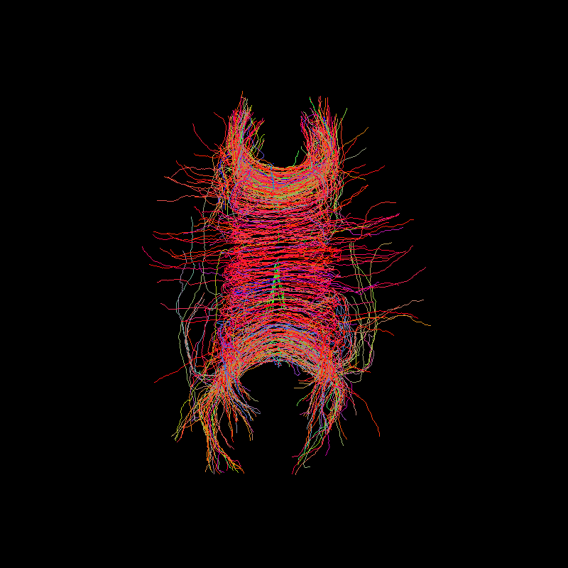
fod = csd_fit.odf(small_sphere)
pmf = fod.clip(min=0)
prob_dg = ProbabilisticDirectionGetter.from_pmf(pmf, max_angle=30.,
                                                sphere=small_sphere)
streamline_generator = LocalTracking(prob_dg, stopping_criterion, seeds,
                                     affine, step_size=.5)
streamlines = Streamlines(streamline_generator)
sft = StatefulTractogram(streamlines, hardi_img, Space.RASMM)
save_trk(sft, "tractogram_probabilistic_dg_pmf.trk")

if has_fury:
    r = window.Renderer()
    r.add(actor.line(streamlines, colormap.line_colors(streamlines)))
    window.record(r, out_path='tractogram_probabilistic_dg_pmf.png',
                  size=(800, 800))
    if interactive:
        window.show(r)

Corpus Callosum using probabilistic direction getter from PMF
One disadvantage of using a discrete PMF to represent possible tracking
directions is that it tends to take up a lot of memory (RAM). The size of the
PMF, the FOD in this case, must be equal to the number of possible tracking
directions on the hemisphere, and every voxel has a unique PMF. In this case
the data is (81, 106, 76) and small_sphere has 181 directions so the
FOD is (81, 106, 76, 181). One way to avoid sampling the PMF and holding it
in memory is to build the direction getter directly from the spherical harmonic
(SH) representation of the FOD. By using this approach, we can also use a
larger sphere, like default_sphere which has 362 directions on the
hemisphere, without having to worry about memory limitations.
from dipy.data import default_sphere

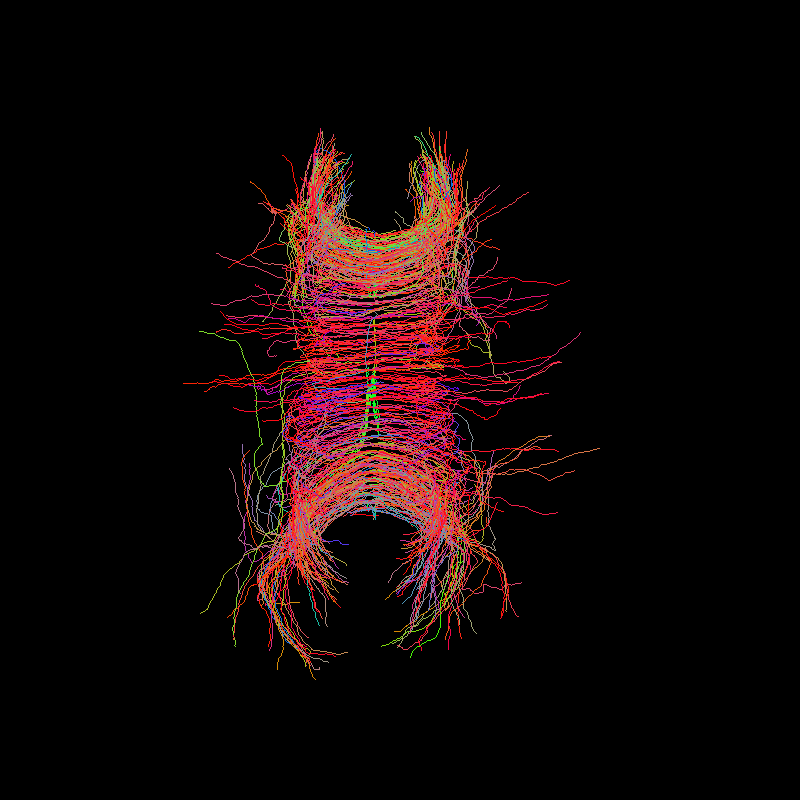
prob_dg = ProbabilisticDirectionGetter.from_shcoeff(csd_fit.shm_coeff,
                                                    max_angle=30.,
                                                    sphere=default_sphere)
streamline_generator = LocalTracking(prob_dg, stopping_criterion, seeds,
                                     affine, step_size=.5)
streamlines = Streamlines(streamline_generator)
sft = StatefulTractogram(streamlines, hardi_img, Space.RASMM)
save_trk(sft, "tractogram_probabilistic_dg_sh.trk")

if has_fury:
    r = window.Renderer()
    r.add(actor.line(streamlines, colormap.line_colors(streamlines)))
    window.record(r, out_path='tractogram_probabilistic_dg_sh.png',
                  size=(800, 800))
    if interactive:
        window.show(r)

Corpus Callosum using probabilistic direction getter from SH
Not all model fits have the shm_coeff attribute because not all models use
this basis to represent the data internally. However we can fit the ODF of any
model to the spherical harmonic basis using the peaks_from_model function.
from dipy.direction import peaks_from_model

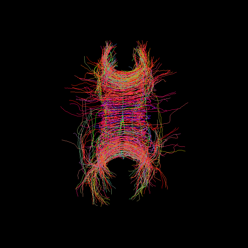
peaks = peaks_from_model(csd_model, data, default_sphere, .5, 25,
                         mask=white_matter, return_sh=True, parallel=True)
fod_coeff = peaks.shm_coeff

prob_dg = ProbabilisticDirectionGetter.from_shcoeff(fod_coeff, max_angle=30.,
                                                    sphere=default_sphere)
streamline_generator = LocalTracking(prob_dg, stopping_criterion, seeds,
                                     affine, step_size=.5)
streamlines = Streamlines(streamline_generator)
sft = StatefulTractogram(streamlines, hardi_img, Space.RASMM)
save_trk(sft, "tractogram_probabilistic_dg_sh_pfm.trk")

if has_fury:
    r = window.Renderer()
    r.add(actor.line(streamlines, colormap.line_colors(streamlines)))
    window.record(r, out_path='tractogram_probabilistic_dg_sh_pfm.png',
                  size=(800, 800))
    if interactive:
        window.show(r)

Corpus Callosum using probabilistic direction getter from SH ( peaks_from_model)
Example source code
You can download the full source code of this example. This same script is also included in the dipy source distribution under the doc/examples/ directory.
