Tracking with the Sparse Fascicle Model
Tracking requires a per-voxel model. Here, the model is the Sparse Fascicle Model (SFM), described in [Rokem2015]. This model reconstructs the diffusion signal as a combination of the signals from different fascicles (see also Reconstruction with the Sparse Fascicle Model).
# Enables/disables interactive visualization
interactive = False

from dipy.data import get_sphere, read_stanford_labels, read_stanford_t1
from dipy.direction.peaks import peaks_from_model
from dipy.io.streamline import save_trk
from dipy.io.stateful_tractogram import Space, StatefulTractogram
from dipy.reconst.csdeconv import auto_response
from dipy.reconst import sfm
from dipy.tracking import utils
from dipy.tracking.local_tracking import LocalTracking
from dipy.tracking.streamline import (select_random_set_of_streamlines,
                                      transform_streamlines,
                                      Streamlines)
from dipy.tracking.stopping_criterion import ThresholdStoppingCriterion
from dipy.viz import window, actor, colormap, has_fury
from numpy.linalg import inv
To begin, we read the Stanford HARDI data set into memory:
hardi_img, gtab, labels_img = read_stanford_labels()
data = hardi_img.get_data()
labels = labels_img.get_data()
affine = hardi_img.affine
This data set provides a label map (generated using FreeSurfer), in which the white matter voxels are labeled as either 1 or 2:
white_matter = (labels == 1) | (labels == 2)
The first step in tracking is generating a model from which tracking directions can be extracted in every voxel.
For the SFM, this requires first that we define a canonical response function that will be used to deconvolve the signal in every voxel
response, ratio = auto_response(gtab, data, roi_radius=10, fa_thr=0.7)
We initialize an SFM model object, using this response function and using the default sphere (362 vertices, symmetrically distributed on the surface of the sphere):
sphere = get_sphere()
sf_model = sfm.SparseFascicleModel(gtab, sphere=sphere,
                                   l1_ratio=0.5, alpha=0.001,
                                   response=response[0])
We fit this model to the data in each voxel in the white-matter mask, so that we can use these directions in tracking:
pnm = peaks_from_model(sf_model, data, sphere,
                       relative_peak_threshold=.5,
                       min_separation_angle=25,
                       mask=white_matter,
                       parallel=True)
A ThresholdStoppingCriterion object is used to segment the data to track only through areas in which the Generalized Fractional Anisotropy (GFA) is sufficiently high.
stopping_criterion = ThresholdStoppingCriterion(pnm.gfa, .25)
Tracking will be started from a set of seeds evenly distributed in the white matter:
seeds = utils.seeds_from_mask(white_matter, affine, density=[2, 2, 2])
For the sake of brevity, we will take only the first 1000 seeds, generating only 1000 streamlines. Remove this line to track from many more points in all of the white matter
seeds = seeds[:1000]
We now have the necessary components to construct a tracking pipeline and execute the tracking
streamline_generator = LocalTracking(pnm, stopping_criterion, seeds, affine,
                                     step_size=.5)
streamlines = Streamlines(streamline_generator)
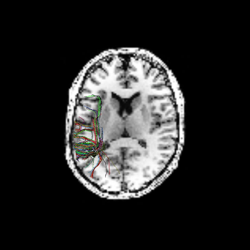
Next, we will create a visualization of these streamlines, relative to this subject’s T1-weighted anatomy:
t1 = read_stanford_t1()
t1_data = t1.get_data()
t1_aff = t1.affine
color = colormap.line_colors(streamlines)
To speed up visualization, we will select a random sub-set of streamlines to display. This is particularly important, if you track from seeds throughout the entire white matter, generating many streamlines. In this case, for demonstration purposes, we subselect 900 streamlines.
plot_streamlines = select_random_set_of_streamlines(streamlines, 900)

if has_fury:
    streamlines_actor = actor.streamtube(
        list(transform_streamlines(plot_streamlines, inv(t1_aff))),
        colormap.line_colors(streamlines), linewidth=0.1)

    vol_actor = actor.slicer(t1_data)

    vol_actor.display(40, None, None)
    vol_actor2 = vol_actor.copy()
    vol_actor2.display(None, None, 35)

    ren = window.Renderer()
    ren.add(streamlines_actor)
    ren.add(vol_actor)
    ren.add(vol_actor2)

    window.record(ren, out_path='tractogram_sfm.png', size=(800, 800))
    if interactive:
        window.show(ren)

Sparse Fascicle Model tracks
Finally, we can save these streamlines to a ‘trk’ file, for use in other software, or for further analysis.
sft = StatefulTractogram(streamlines, hardi_img, Space.RASMM)
save_trk(sft, "tractogram_sfm_detr.trk")
References
- Rokem2015
Ariel Rokem, Jason D. Yeatman, Franco Pestilli, Kendrick N. Kay, Aviv Mezer, Stefan van der Walt, Brian A. Wandell (2015). Evaluating the accuracy of diffusion MRI models in white matter. PLoS ONE 10(4): e0123272. doi:10.1371/journal.pone.0123272
Example source code
You can download the full source code of this example. This same script is also included in the dipy source distribution under the doc/examples/ directory.
