Particle Filtering Tractography

Particle Filtering Tractography (PFT) [Girard2014] uses tissue partial volume estimation (PVE) to reconstruct trajectories connecting the gray matter, and not incorrectly stopping in the white matter or in the corticospinal fluid. It relies on a stopping criterion that identifies the tissue where the streamline stopped. If the streamline correctly stopped in the gray matter, the trajectory is kept. If the streamline incorrectly stopped in the white matter or in the corticospinal fluid, PFT uses anatomical information to find an alternative streamline segment to extend the trajectory. When this segment is found, the tractography continues until the streamline correctly stops in the gray matter.

PFT finds an alternative streamline segment whenever the stopping criterion returns a position classified as ‘INVALIDPOINT’.

This example is an extension of An introduction to the Probabilistic Direction Getter and Using Various Stopping Criterion for Tractography examples. We begin by loading the data, fitting a Constrained Spherical Deconvolution (CSD) reconstruction model, creating the probabilistic direction getter and defining the seeds.

# Enables/disables interactive visualization
interactive = False

import numpy as np

from dipy.data import (read_stanford_labels, default_sphere,
                       read_stanford_pve_maps)
from dipy.direction import ProbabilisticDirectionGetter
from dipy.io.stateful_tractogram import Space, StatefulTractogram
from dipy.io.streamline import save_trk
from dipy.reconst.csdeconv import (ConstrainedSphericalDeconvModel,
                                   auto_response)
from dipy.tracking.local_tracking import (LocalTracking,
                                          ParticleFilteringTracking)
from dipy.tracking.streamline import Streamlines
from dipy.tracking import utils
from dipy.viz import window, actor, colormap, has_fury

img_pve_csf, img_pve_gm, img_pve_wm = read_stanford_pve_maps()
hardi_img, gtab, labels_img = read_stanford_labels()

data = hardi_img.get_data()
labels = labels_img.get_data()
affine = hardi_img.affine
shape = labels.shape

response, ratio = auto_response(gtab, data, roi_radius=10, fa_thr=0.7)
csd_model = ConstrainedSphericalDeconvModel(gtab, response)
csd_fit = csd_model.fit(data, mask=img_pve_wm.get_data())

dg = ProbabilisticDirectionGetter.from_shcoeff(csd_fit.shm_coeff,
                                               max_angle=20.,
                                               sphere=default_sphere)

seed_mask = (labels == 2)
seed_mask[img_pve_wm.get_data() < 0.5] = 0
seeds = utils.seeds_from_mask(seed_mask, affine, density=2)

CMC/ACT Stopping Criterion

Continuous map criterion (CMC) [Girard2014] and Anatomically-constrained tractography (ACT) [Smith2012] both uses PVEs information from anatomical images to determine when the tractography stops. Both stopping criterion use a trilinear interpolation at the tracking position. CMC stopping criterion uses a probability derived from the PVE maps to determine if the streamline reaches a ‘valid’ or ‘invalid’ region. ACT uses a fixed threshold on the PVE maps. Both stopping criterion can be used in conjunction with PFT. In this example, we used CMC.

from dipy.tracking.stopping_criterion import CmcStoppingCriterion

voxel_size = np.average(img_pve_wm.header['pixdim'][1:4])
step_size = 0.2

cmc_criterion = CmcStoppingCriterion.from_pve(img_pve_wm.get_data(),
                                              img_pve_gm.get_data(),
                                              img_pve_csf.get_data(),
                                              step_size=step_size,
                                              average_voxel_size=voxel_size)

# Particle Filtering Tractography
pft_streamline_generator = ParticleFilteringTracking(dg,
                                                     cmc_criterion,
                                                     seeds,
                                                     affine,
                                                     max_cross=1,
                                                     step_size=step_size,
                                                     maxlen=1000,
                                                     pft_back_tracking_dist=2,
                                                     pft_front_tracking_dist=1,
                                                     particle_count=15,
                                                     return_all=False)
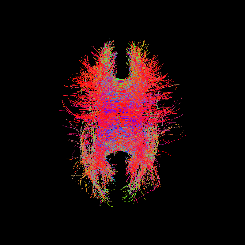
streamlines = Streamlines(pft_streamline_generator)
sft = StatefulTractogram(streamlines, hardi_img, Space.RASMM)
save_trk(sft, "tractogram_pft.trk")

if has_fury:
    r = window.Renderer()
    r.add(actor.line(streamlines, colormap.line_colors(streamlines)))
    window.record(r, out_path='tractogram_pft.png',
                  size=(800, 800))
    if interactive:
        window.show(r)

Corpus Callosum using particle filtering tractography

# Local Probabilistic Tractography
prob_streamline_generator = LocalTracking(dg,
                                          cmc_criterion,
                                          seeds,
                                          affine,
                                          max_cross=1,
                                          step_size=step_size,
                                          maxlen=1000,
                                          return_all=False)
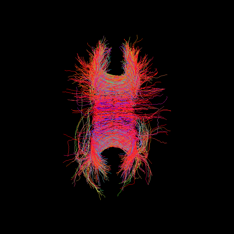
streamlines = Streamlines(prob_streamline_generator)
sft = StatefulTractogram(streamlines, hardi_img, Space.RASMM)
save_trk(sft, "tractogram_probabilistic_cmc.trk")

if has_fury:
    r = window.Renderer()
    r.add(actor.line(streamlines, colormap.line_colors(streamlines)))
    window.record(r, out_path='tractogram_probabilistic_cmc.png',
                  size=(800, 800))
    if interactive:
        window.show(r)

Corpus Callosum using probabilistic tractography

References

Girard2014(1,2)

Girard, G., Whittingstall, K., Deriche, R., & Descoteaux, M. Towards quantitative connectivity analysis: reducing tractography biases. NeuroImage, 98, 266-278, 2014.

Smith2012

Smith, R. E., Tournier, J.-D., Calamante, F., & Connelly, A. Anatomically-constrained tractography: Improved diffusion MRI streamlines tractography through effective use of anatomical information. NeuroImage, 63(3), 1924-1938, 2012.

Example source code

You can download the full source code of this example. This same script is also included in the dipy source distribution under the doc/examples/ directory.