Examples#
Note
The examples here are some uses of the analysis and visualization functionality of DIPY, with example data from actual neuroscience experiments, or with synthetic data, which is generated as part of the example.
All the examples presented in the documentation are generated from fully functioning python scripts, which are available as part of the source distribution in the doc/examples folder.
If you want to replicate a particular analysis or visualization, copy or download the relevant .py script, edit out the body of the text of the example and alter it to your purpose.
Contents
Quick Start#
Preprocessing#
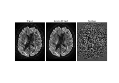
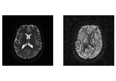
Patch2Self: Self-Supervised Denoising via Statistical Independence
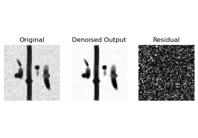
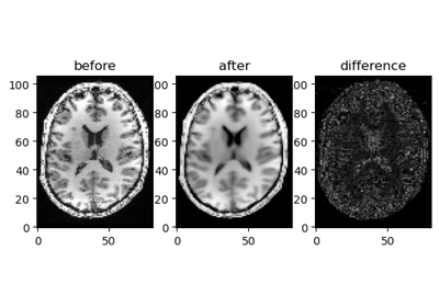
Denoise images using Local PCA via empirical thresholds
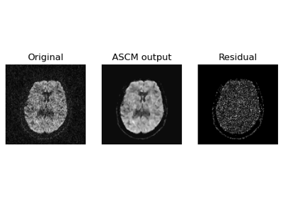
Denoise images using Adaptive Soft Coefficient Matching (ASCM)
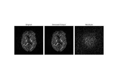
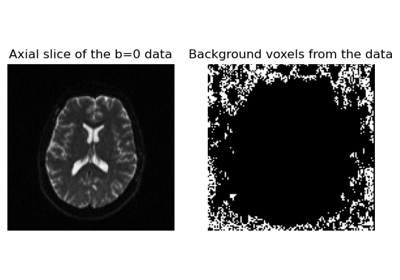
Denoise images using the Marcenko-Pastur PCA algorithm
Reconstruction#
Below, an overview of all reconstruction models available on DIPY.
Note
Some reconstruction models do not have a tutorial yet
Method |
Single Shell |
Multi Shell |
Cartesian |
Paper Data Descriptions |
References |
|---|---|---|---|---|---|
Yes |
Yes |
Yes |
Typical b-value = 1000s/mm^2, maximum b-value 1200s/mm^2 (some success up to 1500s/mm^2) |
||
Yes |
Yes |
Yes |
Typical b-value = 1000s/mm^2, maximum b-value 1200s/mm^2 (some success up to 1500s/mm^2) |
Yendiki2013, Chang2005, Chung2006 |
|
No |
Yes |
No |
DTI-style acquistion, multiple b=0, all shells should be within maximum b-value of 1000 (or 32 directions evenly distributed 500mm/s^2 and 1500mm/s^2 per Henriques 2017) |
||
No |
Yes |
No |
Dual spin echo diffusion-weighted 2D EPI images were acquired with b values of 0, 500, 1000, 1500, 2000, and 2500 s/mm^2 (max b value of 2000 suggested as sufficient in brain tissue); at least 15 directions |
||
No |
Yes |
No |
None |
||
No |
Yes |
No |
DKI-style acquisition: at least two non-zero b shells (max b value 2000), minimum of 15 directions; typically b-values in increments of 500 from 0 to 2000, 30 directions |
||
No |
Yes |
No |
b-values in increments of 500 from 0 to 2000, 30 directions |
||
Yes |
No |
No |
HARDI data (preferably 7T) with at least 200 diffusion images at b=3000 s/mm^2, or multi-shell data with high angular resolution |
||
Westins CSA |
Yes |
No |
No |
||
No |
Yes |
No |
low b-values are needed |
LeBihan 1984 |
|
No |
Yes |
No |
Fadnavis 2019 |
||
SDT |
Yes |
No |
No |
QBI-style acquisition (60-64 directions, b-value 1000mm/s^2) |
Descoteaux 2009 |
No |
No |
Yes |
515 diffusion encodings, b-values from 12,000 to 18,000 s/mm^2. Acceleration in subsequent studies with ~100 diffusion encoding directions in half sphere of the q-space with b-values = 1000, 2000, 3000s/mm2) |
||
No |
No |
Yes |
203 diffusion encodings (isotropic 3D grid points in the q-space contained within a sphere with radius 3.6), maximum b-value=4000mm/s^2 |
||
No |
Yes |
Yes |
Fits any sampling scheme with at least one non-zero b-shell, benefits from more directions. Recommended 23 b-shells ranging from 0 to 4000 in a 258 direction grid-sampling scheme |
Yeh 2010 |
|
Yes |
Yes |
No |
At least 40 directions, b-value above 1000mm/s^2 |
||
Yes |
No |
No |
At least 64 directions, maximum b-values 3000-4000mm/s^2, multi-shell, isotropic voxel size |
||
No |
Yes |
No |
Multi-shell HARDI data (500, 1000, and 2000 s/mm^2; minimum 2 non-zero b-shells) or DSI (514 images in a cube of five lattice-units, one b=0) |
Merlet 2013, Özarslan 2009, Özarslan 2008 |
|
No |
Yes |
No |
Six unit sphere shells with b = 1000, 2000, 3000, 4000, 5000, 6000 s/mm^2 along 19, 32, 56, 87, 125, and 170 directions (see Olson 2019 for candidate sub-sampling schemes) |
||
No |
Yes |
No |
`Tom Dela Haije < https://doi.org/10.1016/j.neuroimage.2019.116405>`__ |
||
MAPL |
No |
Yes |
No |
Multi-shell similar to WU-Minn HCP, with minimum of 60 samples from 2 shells b-value 1000 and 3000s/mm^2 |
|
Yes |
No |
No |
Minimum: 20 gradient directions and a b-value of 1000 s/mm^2; benefits additionally from 60 direction HARDI data with b-value = 3000s/mm^2 or multi-shell |
Tournier 2017, Descoteaux 2008, Tournier 2007 |
|
No |
Yes |
No |
5 b=0, 50 directions at 3 non-zero b-shells: b=1000, b=2000, b=3000 |
||
No |
Yes |
No |
Multi-shell 64 direction b-values of 1000, 2000s/mm^2 as in Alexander 2017. Original model used 1480 s/mm^2 with 92 directions and 36 b=0 |
Anderson 2005, Alexander 2017 |
|
Yes |
Yes |
Yes |
HARDI data with 64 directions at b = 2500s/mm^2, 3 b=0 images (full original acquisition: 256 directions on a sphere at b = 2500s/mm^2, 36 b=0 volumes) |
||
No |
Yes |
No |
Evenly distributed geometric sampling scheme of 216 measurements, 5 b-values (50, 250, 50, 1000, 200mm/s^2), measurement tensors of four shapes: stick, prolate, sphere, and plane |
||
No |
Yes |
No |
At least one b=0, minimum of 39 acquisitions with spherical and linear encoding; optimal 120 (see Morez 2023), ideal 217 see Herberthson 2021 Table 1 |
||
Ball & Stick |
Yes |
Yes |
No |
Three b=0, 60 evenly distributed directions per Jones 1999 at b-value 1000mm/s^2 |
|
No |
Yes |
No |
Minimum 200 volumes of multi-spherical dMRI (multi-shell, multi-diffusion time; varying gradient directions, gradient strengths, and diffusion times) |
Fick 2017 |
|
Power Map |
Yes |
Yes |
No |
HARDI data with 60 directions at b-value = 3000 s/mm^2, 7 b=0 (Minimum: HARDI data with at least 30 directions) |
|
No |
Yes |
No |
72 directions at each of 5 evenly spaced b-values from 0.5 to 2.5 ms/μm2, 5 b-values from 3 to 5 ms/μm2, 5 b-values from 5.5 to 7.5 ms/μm2, and 3 b-values from 8 to 9 ms/μm2 / b=0 ms/μm^-2, and along 33 directions at b-values from 0.2–3 ms/μm^-2 in steps of 0.2 ms/μm^−2 (24 point spherical design and 9 directions identified for rapid kurtosis estimation) |
||
No |
Yes |
No |

Applying positivity constraints to Q-space Trajectory Imaging (QTI+)

Reconstruction of the diffusion signal with the correlation tensor model
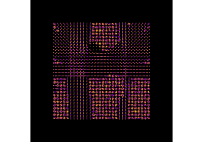
Continuous and analytical diffusion signal modelling with 3D-SHORE
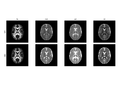
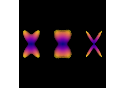
Reconstruction of the diffusion signal with the kurtosis tensor model
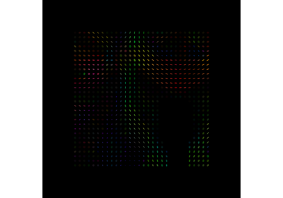
Reconstruction of the diffusion signal with the Tensor model
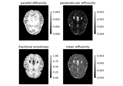
Crossing invariant fiber response function with FORECAST model
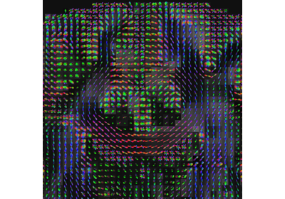
Local reconstruction using the Histological ResDNN
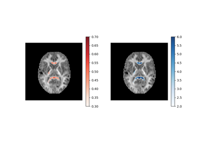
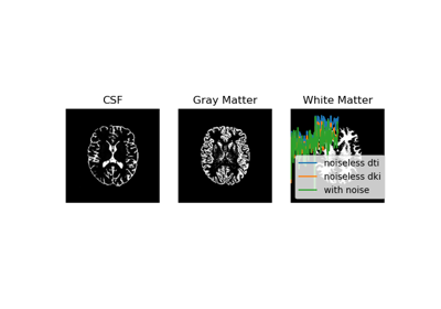
Reconstruction of the diffusion signal with the WMTI model
Using the RESTORE algorithm for robust tensor fitting
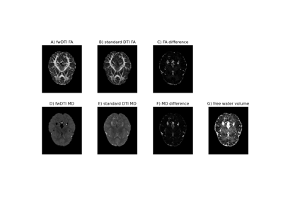
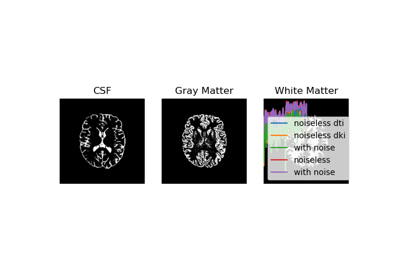
Using the free water elimination model to remove DTI free water contamination
Reconstruction with Constrained Spherical Deconvolution
Continuous and analytical diffusion signal modelling with MAP-MRI
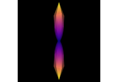
Reconstruction with Robust and Unbiased Model-BAsed Spherical Deconvolution
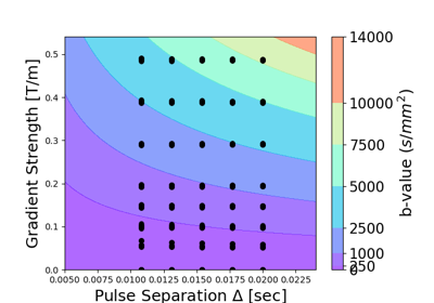
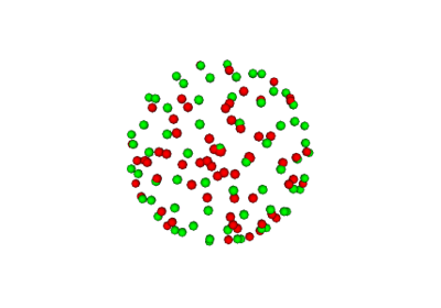
Estimating diffusion time dependent q-space indices using qt-dMRI
Contextual Enhancement#
Fiber Tracking#
An introduction to the Deterministic Maximum Direction Getter
Tracking with Robust Unbiased Model-BAsed Spherical Deconvolution (RUMBA-SD)
Bootstrap and Closest Peak Direction Getters Example
An introduction to the Probabilistic Direction Getter
Streamlines Analysis and Connectivity#
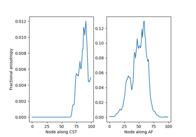
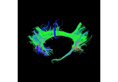
Extracting AFQ tract profiles from segmented bundles
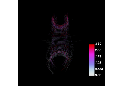
Calculation of Outliers with Cluster Confidence Index
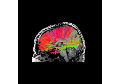
Connectivity Matrices, ROI Intersections and Density Maps
Registration#
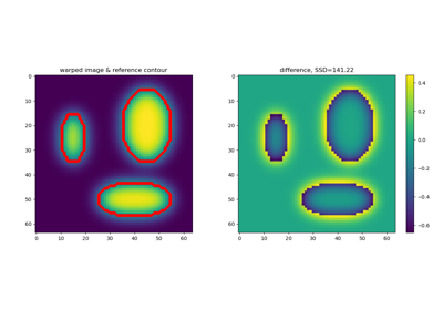
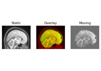
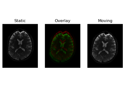
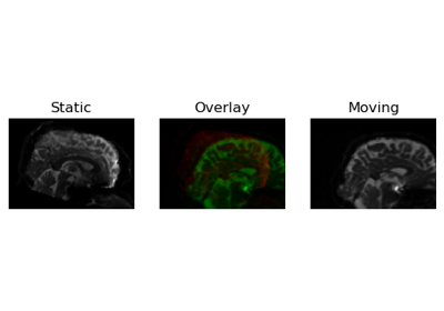
Diffeomorphic Registration with binary and fuzzy images
Segmentation#
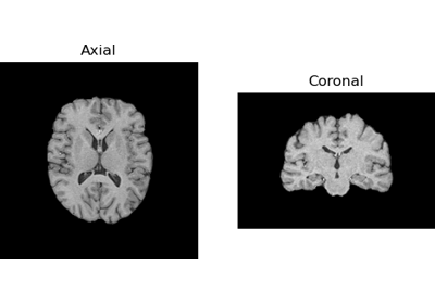
Tissue Classification of a T1-weighted Structural Image
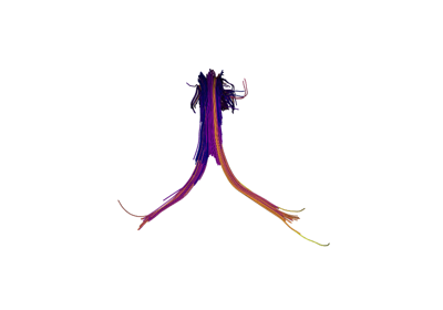
Enhancing QuickBundles with different metrics and features
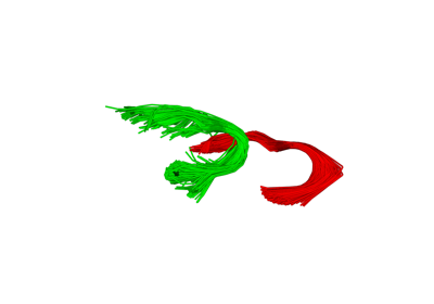
Automatic Fiber Bundle Extraction with RecoBundles
Simulation#
Multiprocessing#
File Formats#
Visualization#
Visualization of ROI Surface Rendered with Streamlines
