Note
Go to the end to download the full example code
Tractography Clustering with QuickBundles#
This example explains how we can use QuickBundles [Garyfallidis12] to simplify/cluster streamlines.
First import the necessary modules.
import numpy as np
from dipy.io.streamline import load_tractogram
from dipy.segment.clustering import QuickBundles
from dipy.io.pickles import save_pickle
from dipy.data import get_fnames
from dipy.viz import window, actor, colormap
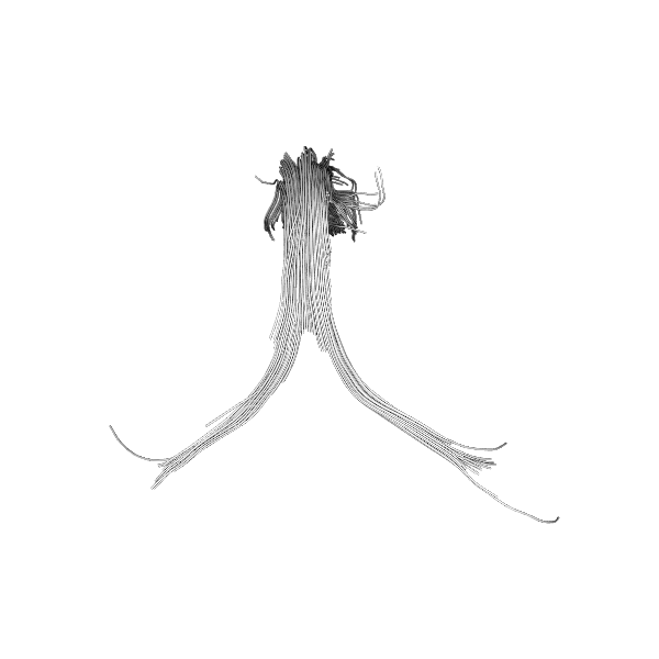
For educational purposes we will try to cluster a small streamline bundle known from neuroanatomy as the fornix.
fname = get_fnames('fornix')
Load fornix streamlines.
fornix = load_tractogram(fname, 'same', bbox_valid_check=False)
streamlines = fornix.streamlines
Perform QuickBundles clustering using the MDF metric and a 10mm distance threshold. Keep in mind that since the MDF metric requires streamlines to have the same number of points, the clustering algorithm will internally use a representation of streamlines that have been automatically downsampled/upsampled so they have only 12 points (To set manually the number of points, see Resample Feature).
qb = QuickBundles(threshold=10.)
clusters = qb.cluster(streamlines)
clusters is a ClusterMap object which contains attributes that provide information about the clustering result.
print("Nb. clusters:", len(clusters))
print("Cluster sizes:", map(len, clusters))
print("Small clusters:", clusters < 10)
print("Streamlines indices of the first cluster:\n", clusters[0].indices)
print("Centroid of the last cluster:\n", clusters[-1].centroid)
Nb. clusters: 4
Cluster sizes: <map object at 0x000001833C7DF6A0>
Small clusters: [False False False  True]
Streamlines indices of the first cluster:
 [0, 7, 8, 10, 11, 12, 13, 14, 15, 18, 26, 30, 33, 35, 41, 65, 66, 85, 100, 101, 105, 115, 116, 119, 122, 123, 124, 125, 126, 128, 129, 135, 139, 142, 143, 144, 148, 151, 159, 167, 175, 180, 181, 185, 200, 208, 210, 224, 237, 246, 249, 251, 256, 267, 270, 280, 284, 293, 296, 297, 299]
Centroid of the last cluster:
 [[ 84.83774  117.9259    77.322784]
 [ 86.108505 115.84363   81.91885 ]
 [ 86.40357  112.25677   85.7293  ]
 [ 86.48337  107.60328   88.137825]
 [ 86.238976 102.51007   89.29447 ]
 [ 85.04564   97.460205  88.542404]
 [ 82.6024    93.14851   86.84209 ]
 [ 78.98937   89.57682   85.63652 ]
 [ 74.72344   86.60828   84.939186]
 [ 70.40846   85.158745  82.4484  ]
 [ 66.745346  86.002625  78.82582 ]
 [ 64.02451   88.43942   75.06974 ]]
clusters also has attributes such as centroids (cluster representatives), and methods like add, remove, and clear to modify the clustering result.
Let’s first show the initial dataset.
# Enables/disables interactive visualization
interactive = False

scene = window.Scene()
scene.SetBackground(1, 1, 1)
scene.add(actor.streamtube(streamlines, window.colors.white))
window.record(scene, out_path='fornix_initial.png', size=(600, 600))
if interactive:
    window.show(scene)

Initial Fornix dataset.
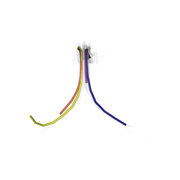
Show the centroids of the fornix after clustering (with random colors):
colormap = colormap.create_colormap(np.arange(len(clusters)))

scene.clear()
scene.SetBackground(1, 1, 1)
scene.add(actor.streamtube(streamlines, window.colors.white, opacity=0.05))
scene.add(actor.streamtube(clusters.centroids, colormap, linewidth=0.4))
window.record(scene, out_path='fornix_centroids.png', size=(600, 600))
if interactive:
    window.show(scene)

Showing the different QuickBundles centroids with random colors.
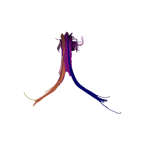
Show the labeled fornix (colors from centroids).
colormap_full = np.ones((len(streamlines), 3))
for cluster, color in zip(clusters, colormap):
    colormap_full[cluster.indices] = color

scene.clear()
scene.SetBackground(1, 1, 1)
scene.add(actor.streamtube(streamlines, colormap_full))
window.record(scene, out_path='fornix_clusters.png', size=(600, 600))
if interactive:
    window.show(scene)

Showing the different clusters.
It is also possible to save the complete ClusterMap object with pickling.
save_pickle('QB.pkl', clusters)
Finally, here is a video of QuickBundles applied on a larger dataset.
# noqa: E501References#
Garyfallidis E. et al., QuickBundles a method for tractography simplification, Frontiers in Neuroscience, vol 6, no 175, 2012.
Total running time of the script: (0 minutes 1.086 seconds)