Calculate SHORE scalar maps

We show how to calculate two SHORE-based scalar maps: return to origin probability (RTOP) [Descoteaux2011] and mean square displacement (MSD) [Wu2007], [Wu2008] on your data. SHORE can be used with any multiple b-value dataset like multi-shell or DSI.

First import the necessary modules:

import numpy as np
import matplotlib.pyplot as plt
from dipy.core.gradients import gradient_table
from dipy.data import get_fnames
from dipy.io.gradients import read_bvals_bvecs
from dipy.io.image import load_nifti
from dipy.reconst.shore import ShoreModel

Download and get the data filenames for this tutorial.

fraw, fbval, fbvec = get_fnames('taiwan_ntu_dsi')

img contains a nibabel Nifti1Image object (data) and gtab contains a GradientTable object (gradient information e.g. b-values). For example, to read the b-values it is possible to write print(gtab.bvals).

Load the raw diffusion data and the affine.

data, affine = load_nifti(fraw)
bvals, bvecs = read_bvals_bvecs(fbval, fbvec)
bvecs[1:] = (bvecs[1:] /
             np.sqrt(np.sum(bvecs[1:] * bvecs[1:], axis=1))[:, None])
gtab = gradient_table(bvals, bvecs)
print('data.shape (%d, %d, %d, %d)' % data.shape)

data.shape (96, 96, 60, 203)

Instantiate the Model.

asm = ShoreModel(gtab)

Let’s just use only one slice only from the data.

dataslice = data[30:70, 20:80, data.shape[2] // 2]

Fit the signal with the model and calculate the SHORE coefficients.

asmfit = asm.fit(dataslice)

  0%|                                                                                                                             | 0/2400 [00:00<?, ?it/s]
  0%|                                                                                                                     | 1/2400 [00:00<12:39,  3.16it/s]
  6%|██████▊                                                                                                           | 143/2400 [00:00<00:05, 434.16it/s]
 11%|████████████▋                                                                                                     | 268/2400 [00:00<00:03, 679.36it/s]
 19%|█████████████████████▌                                                                                           | 457/2400 [00:00<00:01, 1041.85it/s]
 26%|█████████████████████████████▏                                                                                   | 621/2400 [00:00<00:01, 1219.88it/s]
 33%|█████████████████████████████████████▌                                                                           | 798/2400 [00:00<00:01, 1378.96it/s]
 40%|████████████████████████████████████████████▊                                                                    | 953/2400 [00:00<00:01, 1412.92it/s]
 46%|███████████████████████████████████████████████████▋                                                            | 1108/2400 [00:01<00:00, 1445.22it/s]
 53%|███████████████████████████████████████████████████████████▌                                                    | 1276/2400 [00:01<00:00, 1506.70it/s]
 61%|████████████████████████████████████████████████████████████████████▎                                           | 1464/2400 [00:01<00:00, 1608.45it/s]
 70%|█████████████████████████████████████████████████████████████████████████████▉                                  | 1670/2400 [00:01<00:00, 1733.59it/s]
 78%|███████████████████████████████████████████████████████████████████████████████████████▌                        | 1875/2400 [00:01<00:00, 1827.24it/s]
 86%|████████████████████████████████████████████████████████████████████████████████████████████████▏               | 2061/2400 [00:01<00:00, 1763.36it/s]
 93%|████████████████████████████████████████████████████████████████████████████████████████████████████████▌       | 2240/2400 [00:01<00:00, 1579.09it/s]
100%|████████████████████████████████████████████████████████████████████████████████████████████████████████████████| 2400/2400 [00:01<00:00, 1358.82it/s]

Calculate the analytical RTOP on the signal that corresponds to the integral of the signal.

print('Calculating... rtop_signal')
rtop_signal = asmfit.rtop_signal()

Calculating... rtop_signal

Now we calculate the analytical RTOP on the propagator, that corresponds to its central value.

print('Calculating... rtop_pdf')
rtop_pdf = asmfit.rtop_pdf()

Calculating... rtop_pdf

In theory, these two measures must be equal, to show that we calculate the mean square error on this two measures.

mse = np.sum((rtop_signal - rtop_pdf) ** 2) / rtop_signal.size
print(f"MSE = {mse:f}")

MSE = 0.000000

Let’s calculate the analytical mean square displacement on the propagator.

print('Calculating... msd')
msd = asmfit.msd()

Calculating... msd

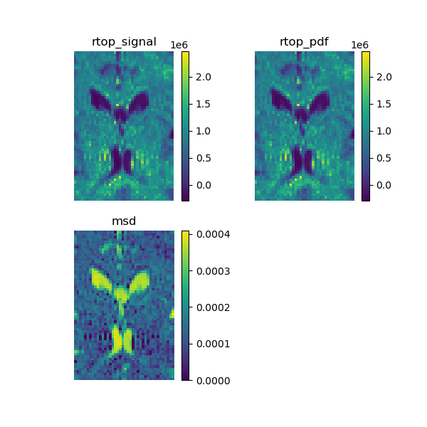
Show the maps and save them to a file.

fig = plt.figure(figsize=(6, 6))
ax1 = fig.add_subplot(2, 2, 1, title='rtop_signal')
ax1.set_axis_off()
ind = ax1.imshow(rtop_signal.T, interpolation='nearest', origin='lower')
plt.colorbar(ind)
ax2 = fig.add_subplot(2, 2, 2, title='rtop_pdf')
ax2.set_axis_off()
ind = ax2.imshow(rtop_pdf.T, interpolation='nearest', origin='lower')
plt.colorbar(ind)
ax3 = fig.add_subplot(2, 2, 3, title='msd')
ax3.set_axis_off()
ind = ax3.imshow(msd.T, interpolation='nearest', origin='lower', vmin=0)
plt.colorbar(ind)
plt.savefig('SHORE_maps.png')

C:\Users\skoudoro\Devel\dipy\doc\examples_revamped\reconstruction\reconst_shore_metrics.py:86: RuntimeWarning: More than 20 figures have been opened. Figures created through the pyplot interface (`matplotlib.pyplot.figure`) are retained until explicitly closed and may consume too much memory. (To control this warning, see the rcParam `figure.max_open_warning`). Consider using `matplotlib.pyplot.close()`.
  fig = plt.figure(figsize=(6, 6))

RTOP and MSD calculated using the SHORE model.

References

[Descoteaux2011]

Descoteaux M. et al., “Multiple q-shell diffusion propagator imaging”, Medical Image Analysis, vol 15, No. 4, p. 603-621, 2011.

[Wu2007]

Wu Y. et al., “Hybrid diffusion imaging”, NeuroImage, vol 36, p. 617-629, 2007.

[Wu2008]

Wu Y. et al., “Computation of Diffusion Function Measures in q-Space Using Magnetic Resonance Hybrid Diffusion Imaging”, IEEE TRANSACTIONS ON MEDICAL IMAGING, vol. 27, No. 6, p. 858-865, 2008.