Note
Go to the end to download the full example code
Gradients and Spheres#
This example shows how you can create gradient tables and sphere objects using DIPY.
Usually, as we saw in Getting started with DIPY, you load your b-values and b-vectors from disk and then you can create your own gradient table. But this time let’s say that you are an MR physicist and you want to design a new gradient scheme or you are a scientist who wants to simulate many different gradient schemes.
Now let’s assume that you are interested in creating a multi-shell acquisition with 2-shells, one at b=1000 \(s/mm^2\) and one at b=2500 \(s/mm^2\). For both shells let’s say that we want a specific number of gradients (64) and we want to have the points on the sphere evenly distributed.
This is possible using the disperse_charges which is an implementation of
electrostatic repulsion [Jones1999].
Let’s start by importing the necessary modules.
import numpy as np
from dipy.core.gradients import gradient_table
from dipy.core.sphere import disperse_charges, Sphere, HemiSphere
from dipy.viz import window, actor
We can first create some random points on a HemiSphere using spherical
polar coordinates.
rng = np.random.default_rng()
n_pts = 64
theta = np.pi * rng.random(n_pts)
phi = 2 * np.pi * rng.random(n_pts)
hsph_initial = HemiSphere(theta=theta, phi=phi)
Next, we call disperse_charges which will iteratively move the points so
that the electrostatic potential energy is minimized.
hsph_updated, potential = disperse_charges(hsph_initial, 5000)
In hsph_updated we have the updated HemiSphere with the points nicely
distributed on the hemisphere. Let’s visualize them.
# Enables/disables interactive visualization
interactive = False

scene = window.Scene()
scene.SetBackground(1, 1, 1)

scene.add(actor.point(hsph_initial.vertices, window.colors.red,
                      point_radius=0.05))
scene.add(actor.point(hsph_updated.vertices, window.colors.green,
                      point_radius=0.05))

window.record(scene, out_path='initial_vs_updated.png', size=(300, 300))
if interactive:
    window.show(scene)
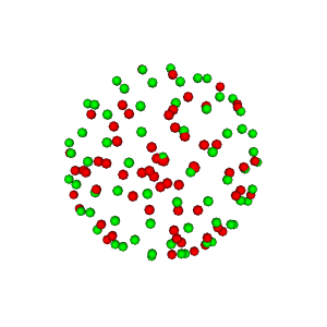
Illustration of electrostatic repulsion of red points which become green points.
We can also create a sphere from the hemisphere and show it in the following way.
sph = Sphere(xyz=np.vstack((hsph_updated.vertices, -hsph_updated.vertices)))

scene.clear()
scene.add(actor.point(sph.vertices, window.colors.green, point_radius=0.05))

window.record(scene, out_path='full_sphere.png', size=(300, 300))
if interactive:
    window.show(scene)

Full sphere.
It is time to create the Gradients. For this purpose we will use the
function gradient_table and fill it with the hsph_updated vectors
that we created above.
vertices = hsph_updated.vertices
values = np.ones(vertices.shape[0])
We need two stacks of vertices, one for every shell, and we need two sets
of b-values, one at 1000 \(s/mm^2\), and one at 2500 \(s/mm^2\), as we discussed
previously.
bvecs = np.vstack((vertices, vertices))
bvals = np.hstack((1000 * values, 2500 * values))
We can also add some b0s. Let’s add one at the beginning and one at the end.
bvecs = np.insert(bvecs, (0, bvecs.shape[0]), np.array([0, 0, 0]), axis=0)
bvals = np.insert(bvals, (0, bvals.shape[0]), 0)

print(bvals)
print(bvecs)
[   0. 1000. 1000. 1000. 1000. 1000. 1000. 1000. 1000. 1000. 1000. 1000.
 1000. 1000. 1000. 1000. 1000. 1000. 1000. 1000. 1000. 1000. 1000. 1000.
 1000. 1000. 1000. 1000. 1000. 1000. 1000. 1000. 1000. 1000. 1000. 1000.
 1000. 1000. 1000. 1000. 1000. 1000. 1000. 1000. 1000. 1000. 1000. 1000.
 1000. 1000. 1000. 1000. 1000. 1000. 1000. 1000. 1000. 1000. 1000. 1000.
 1000. 1000. 1000. 1000. 1000. 2500. 2500. 2500. 2500. 2500. 2500. 2500.
 2500. 2500. 2500. 2500. 2500. 2500. 2500. 2500. 2500. 2500. 2500. 2500.
 2500. 2500. 2500. 2500. 2500. 2500. 2500. 2500. 2500. 2500. 2500. 2500.
 2500. 2500. 2500. 2500. 2500. 2500. 2500. 2500. 2500. 2500. 2500. 2500.
 2500. 2500. 2500. 2500. 2500. 2500. 2500. 2500. 2500. 2500. 2500. 2500.
 2500. 2500. 2500. 2500. 2500. 2500. 2500. 2500. 2500.    0.]
[[ 0.00000000e+00  0.00000000e+00  0.00000000e+00]
 [ 4.27885155e-01 -3.64159326e-01  8.27225652e-01]
 [-7.04956532e-01  4.14476942e-03  7.09238401e-01]
 [ 6.48231836e-03  4.14724759e-02  9.99118618e-01]
 [-2.00922316e-01  9.45151719e-01  2.57523690e-01]
 [ 4.64420512e-01  9.15781188e-02  8.80867207e-01]
 [-4.95126627e-01 -8.65137634e-01  7.99155582e-02]
 [ 2.60252416e-01 -9.00425673e-02  9.61332937e-01]
 [ 6.90254498e-01 -6.27307059e-01  3.60603081e-01]
 [-8.47183356e-01 -2.20574051e-01  4.83350236e-01]
 [ 6.14125513e-01  2.69816089e-01  7.41652973e-01]
 [-3.65810184e-01  7.09091550e-01  6.02803519e-01]
 [ 7.37797281e-01  6.66794736e-01  1.05071178e-01]
 [ 5.30152910e-01 -8.47732225e-01  1.69695667e-02]
 [ 2.43331519e-01 -9.69521432e-01  2.86000650e-02]
 [ 5.22564143e-01 -5.81940542e-01  6.23114694e-01]
 [-2.00411690e-01  5.18859166e-01  8.31035692e-01]
 [ 9.09236625e-01 -4.16271490e-01  2.60896368e-03]
 [ 7.80550544e-01  3.23850748e-01  5.34660211e-01]
 [-3.96064718e-01 -8.52281460e-01  3.41685604e-01]
 [-9.09835740e-01  8.95468440e-02  4.05191670e-01]
 [ 9.51188733e-01  3.00786901e-01  6.90451676e-02]
 [ 7.93070189e-01  5.12520447e-01  3.29184549e-01]
 [-9.66782014e-01  2.01089180e-01  1.57783647e-01]
 [-1.01069525e-01 -9.18025460e-01  3.83424315e-01]
 [-5.11557516e-01  1.80938562e-01  8.39982228e-01]
 [-9.61383543e-01 -1.75562311e-01  2.11942345e-01]
 [-7.07862309e-01 -4.95208621e-01  5.03685788e-01]
 [-7.63824336e-01  6.00533276e-01  2.36499825e-01]
 [-1.32508829e-01 -2.89067045e-01  9.48093695e-01]
 [-1.12065103e-01 -9.91460692e-01  6.66866436e-02]
 [ 2.47163529e-01 -6.20706070e-01  7.44065968e-01]
 [ 1.26151379e-01  5.47377861e-01  8.27322976e-01]
 [-3.01437214e-01 -6.82193078e-03  9.53461624e-01]
 [ 1.97581082e-01  2.82253815e-01  9.38772869e-01]
 [ 7.99438100e-01 -6.43088764e-02  5.97296486e-01]
 [-9.37956803e-02  7.61572643e-01  6.41256174e-01]
 [ 6.13171913e-01 -1.66345739e-01  7.72236557e-01]
 [ 3.53787832e-01  8.38142282e-01  4.15152605e-01]
 [-2.64290833e-01 -7.51043362e-01  6.05048944e-01]
 [ 1.37789170e-01 -3.67265431e-01  9.19853384e-01]
 [-4.47688569e-01 -5.58048740e-01  6.98682008e-01]
 [ 8.71511170e-02 -7.91995691e-01  6.04274365e-01]
 [ 9.20178672e-01 -2.75742692e-01  2.77915777e-01]
 [-4.09793985e-01 -2.64951228e-01  8.72851497e-01]
 [-8.47828696e-01 -5.11290023e-01  1.40602328e-01]
 [-5.17479328e-01  4.49340714e-01  7.28222540e-01]
 [-4.58545459e-01  8.19730483e-01  3.43187991e-01]
 [-1.08331445e-01 -5.73162399e-01  8.12249446e-01]
 [ 5.64081315e-01  6.39019407e-01  5.22940214e-01]
 [ 9.91596059e-01 -1.48597307e-04  1.29372460e-01]
 [ 1.74627718e-01  7.76592265e-01  6.05317780e-01]
 [ 4.64336996e-01  8.67491316e-01  1.78465601e-01]
 [-1.87691754e-01  2.73805354e-01  9.43293397e-01]
 [ 1.94403472e-01 -9.27721773e-01  3.18652792e-01]
 [ 8.59382086e-02  9.55431988e-01  2.82425816e-01]
 [-6.58213108e-01 -6.86074216e-01  3.09931726e-01]
 [ 7.67597364e-01 -3.77106875e-01  5.18251571e-01]
 [-6.33868483e-01 -2.87414687e-01  7.18055391e-01]
 [ 4.46964089e-01 -8.09944164e-01  3.79754597e-01]
 [-7.78018827e-01  2.86908466e-01  5.58900919e-01]
 [ 4.17480219e-01  4.99431568e-01  7.59130012e-01]
 [-6.65355974e-01  5.65040013e-01  4.87884425e-01]
 [ 7.50682215e-01 -6.56091908e-01  7.75862147e-02]
 [ 9.13578748e-01  1.02792752e-01  3.93455869e-01]
 [ 0.00000000e+00  0.00000000e+00  0.00000000e+00]]
Both b-values and b-vectors look correct. Let’s now create the
GradientTable.
gtab = gradient_table(bvals, bvecs)

scene.clear()
We can also visualize the gradients. Let’s color the first shell blue and the second shell cyan.
colors_b1000 = window.colors.blue * np.ones(vertices.shape)
colors_b2500 = window.colors.cyan * np.ones(vertices.shape)
colors = np.vstack((colors_b1000, colors_b2500))
colors = np.insert(colors, (0, colors.shape[0]), np.array([0, 0, 0]), axis=0)
colors = np.ascontiguousarray(colors)

scene.add(actor.point(gtab.gradients, colors, point_radius=100))

window.record(scene, out_path='gradients.png', size=(300, 300))
if interactive:
    window.show(scene)
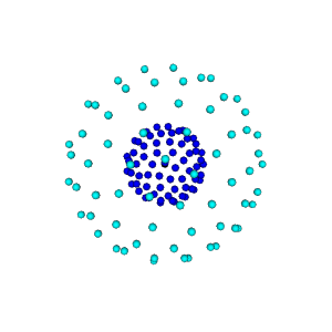
Diffusion gradients.
References#
Jones, DK. et al. Optimal strategies for measuring diffusion in anisotropic systems by magnetic resonance imaging, Magnetic Resonance in Medicine, vol 42, no 3, 515-525, 1999.
Total running time of the script: (0 minutes 4.129 seconds)