Note
Go to the end to download the full example code.
Denoise images using Non-Local Means (NLMEANS)#
Using the non-local means filter [1] and [2] and you can denoise 3D or 4D images and boost the SNR of your datasets. You can also decide between modeling the noise as Gaussian or Rician (default).
We start by loading the necessary modules
from time import time

import matplotlib.pyplot as plt
import numpy as np

from dipy.data import get_fnames
from dipy.denoise.nlmeans import nlmeans
from dipy.denoise.noise_estimate import estimate_sigma
from dipy.io.image import load_nifti, save_nifti
Then, let’s fetch and load a T1 data from Stanford University
t1_fname = get_fnames(name="stanford_t1")
data, affine = load_nifti(t1_fname)

mask = data > 1500

print("vol size", data.shape)
vol size (81, 106, 76)
In order to call non_local_means first you need to estimate the standard
deviation of the noise. We have used N=32 since the Stanford dataset was
acquired on a 3T GE scanner with a 32 array head coil.
sigma = estimate_sigma(data, N=32)
Calling the main function non_local_means
total time 0.032012939453125
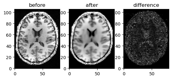
Let us plot the axial slice of the denoised output
axial_middle = data.shape[2] // 2

before = data[:, :, axial_middle].T
after = den[:, :, axial_middle].T

difference = np.abs(after.astype(np.float64) - before.astype(np.float64))

difference[~mask[:, :, axial_middle].T] = 0


fig, ax = plt.subplots(1, 3)
ax[0].imshow(before, cmap="gray", origin="lower")
ax[0].set_title("before")
ax[1].imshow(after, cmap="gray", origin="lower")
ax[1].set_title("after")
ax[2].imshow(difference, cmap="gray", origin="lower")
ax[2].set_title("difference")

plt.savefig("denoised.png", bbox_inches="tight")

Showing axial slice before (left) and after (right) NLMEANS denoising
save_nifti("denoised.nii.gz", den, affine)
An improved version of non-local means denoising is adaptive soft coefficient matching, please refer to Denoise images using Adaptive Soft Coefficient Matching (ASCM) for more details.
References#
Total running time of the script: (0 minutes 0.192 seconds)