Note
Go to the end to download the full example code.
Crossing invariant fiber response function with FORECAST model#
We show how to obtain a voxel specific response function in the form of axially symmetric tensor and the fODF using the FORECAST model from [1], [2] and [3].
First import the necessary modules:
import matplotlib.pyplot as plt
import nibabel as nib
import numpy as np

from dipy.core.gradients import gradient_table
from dipy.data import fetch_hbn, get_sphere
from dipy.reconst.forecast import ForecastModel
from dipy.viz import actor, window
Download and read the data for this tutorial. Our implementation of FORECAST requires multi-shell data.fetch_hbn() provides data that was acquired using b-values of 1000 and 2000 as part of the Healthy Brain Network study [4] and was preprocessed and quality controlled in the HBN-POD2 dataset [5].
data_path = fetch_hbn(["NDARAA948VFH"])[1]
dwi_path = (
    data_path / "derivatives" / "qsiprep" / "sub-NDARAA948VFH" / "ses-HBNsiteRU" / "dwi"
)

img = nib.load(
    dwi_path
    / "sub-NDARAA948VFH_ses-HBNsiteRU_acq-64dir_space-T1w_desc-preproc_dwi.nii.gz",
)

gtab = gradient_table(
    dwi_path
    / "sub-NDARAA948VFH_ses-HBNsiteRU_acq-64dir_space-T1w_desc-preproc_dwi.bval",
    bvecs=(
        dwi_path
        / "sub-NDARAA948VFH_ses-HBNsiteRU_acq-64dir_space-T1w_desc-preproc_dwi.bvec"
    ),
)

data = np.asarray(img.dataobj)

mask_img = nib.load(
    dwi_path
    / "sub-NDARAA948VFH_ses-HBNsiteRU_acq-64dir_space-T1w_desc-brain_mask.nii.gz"
)

brain_mask = mask_img.get_fdata()
Let us consider only a single slice for the FORECAST fitting
data_small = data[:, :, 50:51]
mask_small = brain_mask[:, :, 50:51]
Instantiate the FORECAST Model.
“sh_order_max” is the spherical harmonics order (l) used for the fODF.
dec_alg is the spherical deconvolution algorithm used for the FORECAST basis fitting, in this case we used the Constrained Spherical Deconvolution (CSD) algorithm.
fm = ForecastModel(gtab, sh_order_max=6, dec_alg="CSD")
Fit the FORECAST to the data
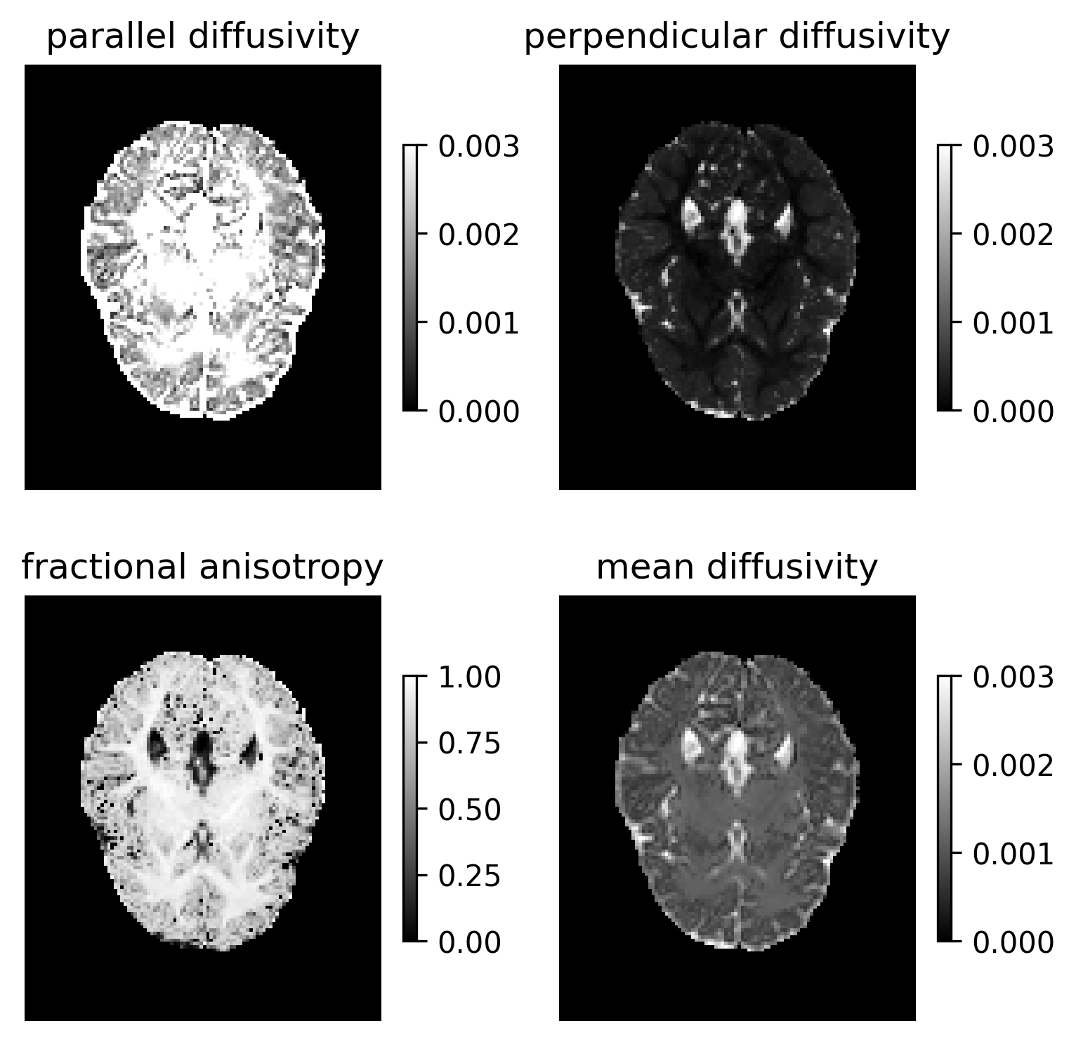
Calculate the crossing invariant tensor indices [2]: the parallel diffusivity, the perpendicular diffusivity, the fractional anisotropy and the mean diffusivity.
d_par = f_fit.dpar
d_perp = f_fit.dperp
fa = f_fit.fractional_anisotropy()
md = f_fit.mean_diffusivity()
Show the indices and save them in FORECAST_indices.png.
fig = plt.figure(figsize=(6, 6))
ax1 = fig.add_subplot(2, 2, 1, title="parallel diffusivity")
ax1.set_axis_off()
ind = ax1.imshow(
    d_par[:, :, 0].T, interpolation="nearest", origin="lower", cmap=plt.cm.gray
)
plt.colorbar(ind, shrink=0.6)
ax2 = fig.add_subplot(2, 2, 2, title="perpendicular diffusivity")
ax2.set_axis_off()
ind = ax2.imshow(
    d_perp[:, :, 0].T, interpolation="nearest", origin="lower", cmap=plt.cm.gray
)
plt.colorbar(ind, shrink=0.6)
ax3 = fig.add_subplot(2, 2, 3, title="fractional anisotropy")
ax3.set_axis_off()
ind = ax3.imshow(
    fa[:, :, 0].T, interpolation="nearest", origin="lower", cmap=plt.cm.gray
)
plt.colorbar(ind, shrink=0.6)
ax4 = fig.add_subplot(2, 2, 4, title="mean diffusivity")
ax4.set_axis_off()
ind = ax4.imshow(
    md[:, :, 0].T, interpolation="nearest", origin="lower", cmap=plt.cm.gray
)
plt.colorbar(ind, shrink=0.6)
plt.savefig("FORECAST_indices.png", dpi=300, bbox_inches="tight")

FORECAST scalar indices.
Load an ODF reconstruction sphere
sphere = get_sphere(name="repulsion724")
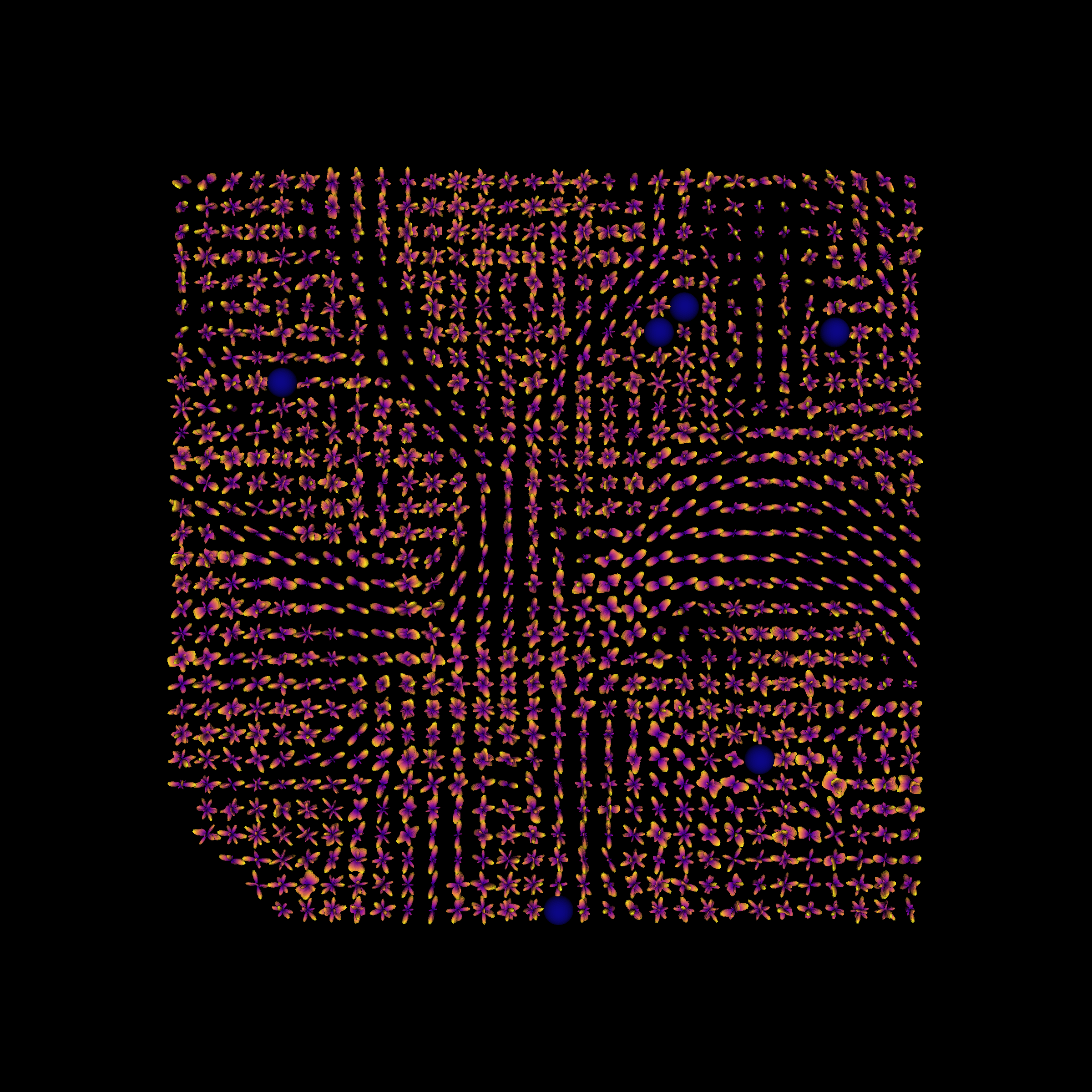
Compute the fODFs.
fODF.shape (108, 129, 1, 724)
Display a part of the fODFs

Fiber Orientation Distribution Functions, in a small ROI of the brain.
References#
Total running time of the script: (1 minutes 4.886 seconds)