Gradients and Spheres

This example shows how you can create gradient tables and sphere objects using DIPY.

Usually, as we saw in Getting started with DIPY, you load your b-values and b-vectors from disk and then you can create your own gradient table. But this time let’s say that you are an MR physicist and you want to design a new gradient scheme or you are a scientist who wants to simulate many different gradient schemes.

Now let’s assume that you are interested in creating a multi-shell acquisition with 2-shells, one at b=1000 \(s/mm^2\) and one at b=2500 \(s/mm^2\). For both shells let’s say that we want a specific number of gradients (64) and we want to have the points on the sphere evenly distributed.

This is possible using the dipy.core.sphere.disperse_charges() which is an implementation of electrostatic repulsion Jones et al.[1] .

Let’s start by importing the necessary modules.

import numpy as np

from dipy.core.gradients import gradient_table
from dipy.core.sphere import HemiSphere, Sphere, disperse_charges
from dipy.viz import actor, window

We can first create some random points on a HemiSphere using spherical polar coordinates.

rng = np.random.default_rng()
n_pts = 64
theta = np.pi * rng.random(n_pts)
phi = 2 * np.pi * rng.random(n_pts)
hsph_initial = HemiSphere(theta=theta, phi=phi)

Next, we call dipy.core.sphere.disperse_charges() which will iteratively move the points so that the electrostatic potential energy is minimized.

hsph_updated, potential = disperse_charges(hsph_initial, 5000)

In hsph_updated we have the updated HemiSphere with the points nicely distributed on the hemisphere. Let’s visualize them.

# Enables/disables interactive visualization
interactive = False

scene = window.Scene()
scene.SetBackground(1, 1, 1)

scene.add(actor.point(hsph_initial.vertices, window.colors.red, point_radius=0.05))
scene.add(actor.point(hsph_updated.vertices, window.colors.green, point_radius=0.05))

window.record(scene=scene, out_path="initial_vs_updated.png", size=(300, 300))
if interactive:
    window.show(scene)

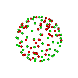
Illustration of electrostatic repulsion of red points which become green points.

We can also create a sphere from the hemisphere and show it in the following way.

sph = Sphere(xyz=np.vstack((hsph_updated.vertices, -hsph_updated.vertices)))

scene.clear()
scene.add(actor.point(sph.vertices, window.colors.green, point_radius=0.05))

window.record(scene=scene, out_path="full_sphere.png", size=(300, 300))
if interactive:
    window.show(scene)

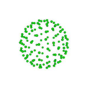
Full sphere.

It is time to create the Gradients. For this purpose we will use the function gradient_table and fill it with the hsph_updated vectors that we created above.

vertices = hsph_updated.vertices
values = np.ones(vertices.shape[0])

We need two stacks of vertices, one for every shell, and we need two sets of b-values, one at 1000 \(s/mm^2\), and one at 2500 \(s/mm^2\), as we discussed previously.

bvecs = np.vstack((vertices, vertices))
bvals = np.hstack((1000 * values, 2500 * values))

We can also add some b0s. Let’s add one at the beginning and one at the end.

bvecs = np.insert(bvecs, (0, bvecs.shape[0]), np.array([0, 0, 0]), axis=0)
bvals = np.insert(bvals, (0, bvals.shape[0]), 0)

print(bvals)
print(bvecs)

[   0. 1000. 1000. 1000. 1000. 1000. 1000. 1000. 1000. 1000. 1000. 1000.
 1000. 1000. 1000. 1000. 1000. 1000. 1000. 1000. 1000. 1000. 1000. 1000.
 1000. 1000. 1000. 1000. 1000. 1000. 1000. 1000. 1000. 1000. 1000. 1000.
 1000. 1000. 1000. 1000. 1000. 1000. 1000. 1000. 1000. 1000. 1000. 1000.
 1000. 1000. 1000. 1000. 1000. 1000. 1000. 1000. 1000. 1000. 1000. 1000.
 1000. 1000. 1000. 1000. 1000. 2500. 2500. 2500. 2500. 2500. 2500. 2500.
 2500. 2500. 2500. 2500. 2500. 2500. 2500. 2500. 2500. 2500. 2500. 2500.
 2500. 2500. 2500. 2500. 2500. 2500. 2500. 2500. 2500. 2500. 2500. 2500.
 2500. 2500. 2500. 2500. 2500. 2500. 2500. 2500. 2500. 2500. 2500. 2500.
 2500. 2500. 2500. 2500. 2500. 2500. 2500. 2500. 2500. 2500. 2500. 2500.
 2500. 2500. 2500. 2500. 2500. 2500. 2500. 2500. 2500.    0.]
[[ 0.          0.          0.        ]
 [-0.09108729  0.2360898   0.96745269]
 [-0.22690291 -0.77230991  0.5933401 ]
 [ 0.00945267 -0.93379308  0.3576886 ]
 [-0.74870532 -0.40039548  0.52832169]
 [-0.46556961  0.88464141  0.02558323]
 [ 0.45922737 -0.68069152  0.57076202]
 [ 0.13305385 -0.77941838  0.6122121 ]
 [-0.13510586 -0.98948015  0.05172473]
 [ 0.07730184 -0.33730943  0.93821467]
 [-0.0248746   0.9697912   0.24266494]
 [ 0.43408028  0.16188586  0.8862095 ]
 [ 0.70248441  0.61877059  0.35162284]
 [ 0.71484446 -0.51634747  0.47157469]
 [-0.55544932 -0.81145582  0.18170167]
 [-0.59380515  0.71532748  0.36837758]
 [-0.6372125   0.21431328  0.74029052]
 [ 0.3386335   0.92818392  0.15427885]
 [-0.94183671 -0.33502481  0.02649496]
 [ 0.88152234  0.36806833  0.29570942]
 [ 0.90656485 -0.26754297  0.32643671]
 [ 0.69054248  0.39819398  0.60381507]
 [-0.14462319 -0.10123318  0.98429466]
 [-0.70817151  0.70024479  0.09027929]
 [-0.26439427 -0.39755728  0.87866027]
 [ 0.32310672 -0.88206863  0.34286584]
 [-0.06949965 -0.60736083  0.7913802 ]
 [ 0.58780755  0.79898776  0.12688911]
 [ 0.82023715 -0.54843619  0.16256928]
 [ 0.15972573  0.00707144  0.9871361 ]
 [ 0.21372355  0.66590314  0.71476937]
 [ 0.38385633 -0.20129894  0.90118425]
 [ 0.63838639  0.00219429  0.76971294]
 [ 0.45560803  0.45655077  0.76418761]
 [-0.83066399  0.03980373  0.55534943]
 [-0.94712619  0.12487103  0.29556589]
 [-0.99852771 -0.03993768  0.03670682]
 [-0.31932419  0.89551096  0.30998738]
 [ 0.96347904 -0.26633673  0.02780075]
 [-0.49795729 -0.48574321  0.71839549]
 [ 0.18681056 -0.98090799  0.05404935]
 [ 0.96043187  0.05040322  0.27391628]
 [-0.76664664 -0.57531072  0.28507983]
 [-0.34260899  0.46138497  0.81837826]
 [-0.32898908  0.72972368  0.59939097]
 [ 0.7890586  -0.18749769  0.58500525]
 [-0.91587051 -0.22702353  0.3311216 ]
 [-0.06231592  0.57136242  0.81832861]
 [-0.68540622 -0.16480446  0.70926568]
 [ 0.82624518  0.13859322  0.54599526]
 [-0.04922734  0.82460102  0.56356883]
 [-0.30081743 -0.90421524  0.30315618]
 [-0.45417026 -0.13558296  0.8805377 ]
 [ 0.23028031  0.87177016  0.43242081]
 [ 0.27903228 -0.53618306  0.79664843]
 [-0.86744457  0.45704575  0.19659376]
 [ 0.18265859  0.3624557   0.91392653]
 [-0.51911569 -0.69552275  0.49675647]
 [ 0.56835655 -0.37902544  0.73028115]
 [-0.38557881  0.16222718  0.90830134]
 [ 0.8021835   0.59673693  0.02016613]
 [ 0.59443847 -0.76328128  0.25307031]
 [-0.79326903  0.38184588  0.47425518]
 [-0.57751763  0.5273041   0.62323653]
 [ 0.47618242  0.70937695  0.51964858]
 [-0.09108729  0.2360898   0.96745269]
 [-0.22690291 -0.77230991  0.5933401 ]
 [ 0.00945267 -0.93379308  0.3576886 ]
 [-0.74870532 -0.40039548  0.52832169]
 [-0.46556961  0.88464141  0.02558323]
 [ 0.45922737 -0.68069152  0.57076202]
 [ 0.13305385 -0.77941838  0.6122121 ]
 [-0.13510586 -0.98948015  0.05172473]
 [ 0.07730184 -0.33730943  0.93821467]
 [-0.0248746   0.9697912   0.24266494]
 [ 0.43408028  0.16188586  0.8862095 ]
 [ 0.70248441  0.61877059  0.35162284]
 [ 0.71484446 -0.51634747  0.47157469]
 [-0.55544932 -0.81145582  0.18170167]
 [-0.59380515  0.71532748  0.36837758]
 [-0.6372125   0.21431328  0.74029052]
 [ 0.3386335   0.92818392  0.15427885]
 [-0.94183671 -0.33502481  0.02649496]
 [ 0.88152234  0.36806833  0.29570942]
 [ 0.90656485 -0.26754297  0.32643671]
 [ 0.69054248  0.39819398  0.60381507]
 [-0.14462319 -0.10123318  0.98429466]
 [-0.70817151  0.70024479  0.09027929]
 [-0.26439427 -0.39755728  0.87866027]
 [ 0.32310672 -0.88206863  0.34286584]
 [-0.06949965 -0.60736083  0.7913802 ]
 [ 0.58780755  0.79898776  0.12688911]
 [ 0.82023715 -0.54843619  0.16256928]
 [ 0.15972573  0.00707144  0.9871361 ]
 [ 0.21372355  0.66590314  0.71476937]
 [ 0.38385633 -0.20129894  0.90118425]
 [ 0.63838639  0.00219429  0.76971294]
 [ 0.45560803  0.45655077  0.76418761]
 [-0.83066399  0.03980373  0.55534943]
 [-0.94712619  0.12487103  0.29556589]
 [-0.99852771 -0.03993768  0.03670682]
 [-0.31932419  0.89551096  0.30998738]
 [ 0.96347904 -0.26633673  0.02780075]
 [-0.49795729 -0.48574321  0.71839549]
 [ 0.18681056 -0.98090799  0.05404935]
 [ 0.96043187  0.05040322  0.27391628]
 [-0.76664664 -0.57531072  0.28507983]
 [-0.34260899  0.46138497  0.81837826]
 [-0.32898908  0.72972368  0.59939097]
 [ 0.7890586  -0.18749769  0.58500525]
 [-0.91587051 -0.22702353  0.3311216 ]
 [-0.06231592  0.57136242  0.81832861]
 [-0.68540622 -0.16480446  0.70926568]
 [ 0.82624518  0.13859322  0.54599526]
 [-0.04922734  0.82460102  0.56356883]
 [-0.30081743 -0.90421524  0.30315618]
 [-0.45417026 -0.13558296  0.8805377 ]
 [ 0.23028031  0.87177016  0.43242081]
 [ 0.27903228 -0.53618306  0.79664843]
 [-0.86744457  0.45704575  0.19659376]
 [ 0.18265859  0.3624557   0.91392653]
 [-0.51911569 -0.69552275  0.49675647]
 [ 0.56835655 -0.37902544  0.73028115]
 [-0.38557881  0.16222718  0.90830134]
 [ 0.8021835   0.59673693  0.02016613]
 [ 0.59443847 -0.76328128  0.25307031]
 [-0.79326903  0.38184588  0.47425518]
 [-0.57751763  0.5273041   0.62323653]
 [ 0.47618242  0.70937695  0.51964858]
 [ 0.          0.          0.        ]]

Both b-values and b-vectors look correct. Let’s now create the GradientTable.

gtab = gradient_table(bvals, bvecs=bvecs)

scene.clear()

We can also visualize the gradients. Let’s color the first shell blue and the second shell cyan.

colors_b1000 = window.colors.blue * np.ones(vertices.shape)
colors_b2500 = window.colors.cyan * np.ones(vertices.shape)
colors = np.vstack((colors_b1000, colors_b2500))
colors = np.insert(colors, (0, colors.shape[0]), np.array([0, 0, 0]), axis=0)
colors = np.ascontiguousarray(colors)

scene.add(actor.point(gtab.gradients, colors, point_radius=100))

window.record(scene=scene, out_path="gradients.png", size=(300, 300))
if interactive:
    window.show(scene)

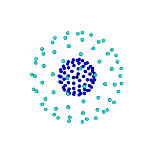
Diffusion gradients.

References

[1]

Derek K. Jones, Mark A. Horsfield, and Andrew Simmons. Optimal strategies for measuring diffusion in anisotropic systems by magnetic resonance imaging. Magnetic Resonance in Medicine, 42(3):515–25, 1999. URL: http://www.ncbi.nlm.nih.gov/pubmed/10467296, doi:10.1002/(SICI)1522-2594(199909)42:3<515::AID-MRM14>3.0.CO;2-Q.