Note
Go to the end to download the full example code.
Symmetric Diffeomorphic Registration in 3D#
This example explains how to register 3D volumes using the Symmetric Normalization (SyN) algorithm proposed by Avants et al.[1] (also implemented in the ANTs software [2])
We will register two 3D volumes from the same modality using SyN with the Cross -Correlation (CC) metric.
import numpy as np

from dipy.align import read_mapping, write_mapping
from dipy.align.imaffine import AffineMap
from dipy.align.imwarp import SymmetricDiffeomorphicRegistration
from dipy.align.metrics import CCMetric
from dipy.data import get_fnames
from dipy.io.image import load_nifti
from dipy.segment.mask import median_otsu
from dipy.viz import regtools
Let’s fetch two b0 volumes, the first one will be the b0 from the Stanford HARDI dataset
hardi_fname, hardi_bval_fname, hardi_bvec_fname = get_fnames(name="stanford_hardi")

stanford_b0, stanford_b0_affine = load_nifti(hardi_fname)
stanford_b0 = np.squeeze(stanford_b0)[..., 0]
The second one will be the same b0 we used for the 2D registration tutorial
t1_fname, b0_fname = get_fnames(name="syn_data")
syn_b0, syn_b0_affine = load_nifti(b0_fname)
We first remove the skull from the b0’s
stanford_b0_masked, stanford_b0_mask = median_otsu(
    stanford_b0, median_radius=4, numpass=4
)
syn_b0_masked, syn_b0_mask = median_otsu(syn_b0, median_radius=4, numpass=4)

static = stanford_b0_masked
static_affine = stanford_b0_affine
moving = syn_b0_masked
moving_affine = syn_b0_affine
Suppose we have already done a linear registration to roughly align the two images
pre_align = np.array(
    [
        [1.02783543e00, -4.83019053e-02, -6.07735639e-02, -2.57654118e00],
        [4.34051706e-03, 9.41918267e-01, -2.66525861e-01, 3.23579799e01],
        [5.34288908e-02, 2.90262026e-01, 9.80820307e-01, -1.46216651e01],
        [0.00000000e00, 0.00000000e00, 0.00000000e00, 1.00000000e00],
    ]
)
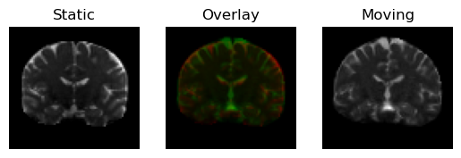
As we did in the 2D example, we would like to visualize (some slices of) the two volumes by overlapping them over two channels of a color image. To do that we need them to be sampled on the same grid, so let’s first re-sample the moving image on the static grid. We create an AffineMap to transform the moving image towards the static image
affine_map = AffineMap(
    pre_align,
    domain_grid_shape=static.shape,
    domain_grid2world=static_affine,
    codomain_grid_shape=moving.shape,
    codomain_grid2world=moving_affine,
)

resampled = affine_map.transform(moving)
plot the overlapped middle slices of the volumes
regtools.overlay_slices(
    static,
    resampled,
    slice_index=None,
    slice_type=1,
    ltitle="Static",
    rtitle="Moving",
    fname="input_3d.png",
)

<Figure size 640x480 with 3 Axes>
Static image in red on top of the pre-aligned moving image (in green).
We want to find an invertible map that transforms the moving image into the static image. We will use the Cross-Correlation metric
Now we define an instance of the registration class. The SyN algorithm uses a multi-resolution approach by building a Gaussian Pyramid. We instruct the registration object to perform at most \([n_0, n_1, ..., n_k]\) iterations at each level of the pyramid. The 0-th level corresponds to the finest resolution.
level_iters = [10, 10, 5]
sdr = SymmetricDiffeomorphicRegistration(metric, level_iters=level_iters)
Execute the optimization, which returns a DiffeomorphicMap object, that can be used to register images back and forth between the static and moving domains. We provide the pre-aligning matrix that brings the moving image closer to the static image
mapping = sdr.optimize(
    static,
    moving,
    static_grid2world=static_affine,
    moving_grid2world=moving_affine,
    prealign=pre_align,
)
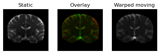
Now let’s warp the moving image and see if it gets similar to the static image
warped_moving = mapping.transform(moving)
We plot the overlapped middle slices
regtools.overlay_slices(
    static,
    warped_moving,
    slice_index=None,
    slice_type=1,
    ltitle="Static",
    rtitle="Warped moving",
    fname="warped_moving.png",
)

<Figure size 640x480 with 3 Axes>
Moving image transformed under the (direct) transformation in green on top of the static image (in red).
And we can also apply the inverse mapping to verify that the warped static image is similar to the moving image
warped_static = mapping.transform_inverse(static)
regtools.overlay_slices(
    warped_static,
    moving,
    slice_index=None,
    slice_type=1,
    ltitle="Warped static",
    rtitle="Moving",
    fname="warped_static.png",
)

<Figure size 640x480 with 3 Axes>
Static image transformed under the (inverse) transformation in red on top of the moving image (in green). Note that the moving image has a lower resolution.
If you wish, you can also save the transformation to a file, so that it can be applied to other images in the future. This can be done with the write_mapping function. The data in the file will be organized with shape (X, Y, Z, 3, 2), such that the forward mapping in each voxel is in data[i, j, k, :, 0] and the backward mapping in each voxel is in data[i, j, k, :, 1]
write_mapping(mapping, "mapping.nii.gz")
# To read the mapping back, use the `read_mapping` function
saved_mapping = read_mapping("mapping.nii.gz", hardi_fname, b0_fname)
References#
Total running time of the script: (0 minutes 37.624 seconds)