Note
Go to the end to download the full example code.
Reconstruction of the diffusion signal with the WMTI model (DKI-MICRO)#
DKI can also be used to derive concrete biophysical parameters by applying microstructural models to DT and KT estimated from DKI. For instance, Fieremans et al.[1] showed that DKI can be used to estimate the contribution of hindered and restricted diffusion for well-aligned fibers - a model that was later referred to as the white matter tract integrity (WMTI) technique [2]. The two tensors of WMTI can be also interpreted as the influences of intra- and extra-cellular compartments and can be used to estimate the axonal volume fraction and diffusion extra-cellular tortuosity. According to previous studies [3], [2] these latter measures can be used to distinguish processes of axonal loss from processes of myelin degeneration. Details on the implementation of WMTI in DIPY are described in [4].
In this example, we show how to process a dMRI dataset using the WMTI model.
First, we import all relevant modules:
import matplotlib.pyplot as plt
import numpy as np
from scipy.ndimage import gaussian_filter

from dipy.core.gradients import gradient_table
from dipy.data import get_fnames
from dipy.io.gradients import read_bvals_bvecs
from dipy.io.image import load_nifti
import dipy.reconst.dki as dki
import dipy.reconst.dki_micro as dki_micro
from dipy.segment.mask import median_otsu
As the standard DKI, WMTI requires multi-shell data, i.e. data acquired from more than one non-zero b-value. Here, we use a fetcher to download a multi-shell dataset which was kindly provided by Hansen and Jespersen (more details about the data are provided in their paper [5]).
fraw, fbval, fbvec, t1_fname = get_fnames(name="cfin_multib")

data, affine = load_nifti(fraw)
bvals, bvecs = read_bvals_bvecs(fbval, fbvec)
gtab = gradient_table(bvals, bvecs=bvecs)
For comparison, this dataset is pre-processed using the same steps used in the example for reconstructing DKI (see Reconstruction of the diffusion signal with the kurtosis tensor model (DKI)).
# data masking
maskdata, mask = median_otsu(data, vol_idx=[0, 1], median_radius=4, numpass=2, dilate=1)

# Smoothing
fwhm = 1.25
gauss_std = fwhm / np.sqrt(8 * np.log(2))
data_smooth = np.zeros(data.shape)
for v in range(data.shape[-1]):
    data_smooth[..., v] = gaussian_filter(data[..., v], sigma=gauss_std)
The WMTI model can be defined in DIPY by instantiating the ‘KurtosisMicrostructureModel’ object in the following way:
Before fitting this microstructural model, it is useful to indicate the regions in which this model provides meaningful information (i.e. voxels of well-aligned fibers). Following Fieremans et al.[1], a simple way to select this region is to generate a well-aligned fiber mask based on the values of diffusion sphericity, planarity and linearity. Here we will follow these selection criteria for a better comparison of our figures with the original article published by Fieremans et al.[1]. Nevertheless, it is important to note that voxels with well-aligned fibers can be selected based on other approaches such as using predefined regions of interest.
# Diffusion Tensor is computed based on the standard DKI model
dkimodel = dki.DiffusionKurtosisModel(gtab)
dkifit = dkimodel.fit(data_smooth, mask=mask)

# Initialize well aligned mask with ones
well_aligned_mask = np.ones(data.shape[:-1], dtype="bool")

# Diffusion coefficient of linearity (cl) has to be larger than 0.4, thus
# we exclude voxels with cl < 0.4.
cl = dkifit.linearity.copy()
well_aligned_mask[cl < 0.4] = False

# Diffusion coefficient of planarity (cp) has to be lower than 0.2, thus
# we exclude voxels with cp > 0.2.
cp = dkifit.planarity.copy()
well_aligned_mask[cp > 0.2] = False

# Diffusion coefficient of sphericity (cs) has to be lower than 0.35, thus
# we exclude voxels with cs > 0.35.
cs = dkifit.sphericity.copy()
well_aligned_mask[cs > 0.35] = False

# Removing nan associated with background voxels
well_aligned_mask[np.isnan(cl)] = False
well_aligned_mask[np.isnan(cp)] = False
well_aligned_mask[np.isnan(cs)] = False
Analogous to DKI, the data fit can be done by calling the fit function of
the model’s object as follows:
dki_micro_fit = dki_micro_model.fit(data_smooth, mask=well_aligned_mask)
The KurtosisMicrostructureFit object created by this fit function can
then be used to extract model parameters such as the axonal water fraction
and diffusion hindered tortuosity:
AWF = dki_micro_fit.awf
TORT = dki_micro_fit.tortuosity
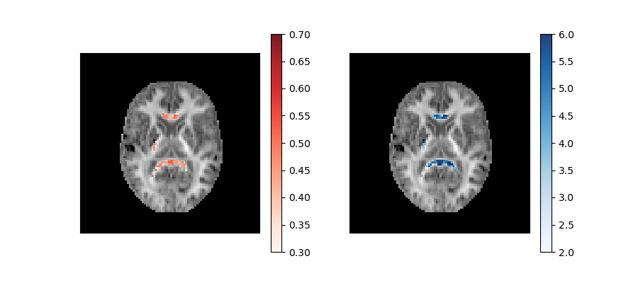
These parameters are plotted below on top of the mean kurtosis maps:
MK = dkifit.mk(min_kurtosis=0, max_kurtosis=3)

axial_slice = 9

fig1, ax = plt.subplots(1, 2, figsize=(9, 4), subplot_kw={"xticks": [], "yticks": []})

AWF[AWF == 0] = np.nan
TORT[TORT == 0] = np.nan

ax[0].imshow(
    MK[:, :, axial_slice].T, cmap=plt.cm.gray, interpolation="nearest", origin="lower"
)
im0 = ax[0].imshow(
    AWF[:, :, axial_slice].T,
    cmap=plt.cm.Reds,
    alpha=0.9,
    vmin=0.3,
    vmax=0.7,
    interpolation="nearest",
    origin="lower",
)
fig1.colorbar(im0, ax=ax.flat[0])

ax[1].imshow(
    MK[:, :, axial_slice].T, cmap=plt.cm.gray, interpolation="nearest", origin="lower"
)
im1 = ax[1].imshow(
    TORT[:, :, axial_slice].T,
    cmap=plt.cm.Blues,
    alpha=0.9,
    vmin=2,
    vmax=6,
    interpolation="nearest",
    origin="lower",
)
fig1.colorbar(im1, ax=ax.flat[1])

fig1.savefig("Kurtosis_Microstructural_measures.png")

Axonal water fraction (left panel) and tortuosity (right panel) values of well-aligned fiber regions overlaid on a top of a mean kurtosis all-brain image.
References#
Total running time of the script: (1 minutes 0.519 seconds)