Note
Go to the end to download the full example code.
Reconstruction of Bingham Functions from ODFs#
This example shows how to reconstruct Bingham functions from orientation distribution functions (ODFs). Reconstructed Bingham functions can be useful to quantify properties from ODFs such as fiber dispersion [1], [2].
To begin, let us import the relevant functions and load data consisting of 10 b0s and 150 non-b0s with a b-value of 2000s/mm2.
from dipy.core.gradients import gradient_table
from dipy.core.sphere import unit_icosahedron
from dipy.data import get_fnames
from dipy.io.gradients import read_bvals_bvecs
from dipy.io.image import load_nifti
from dipy.reconst.bingham import sf_to_bingham, sh_to_bingham
from dipy.reconst.csdeconv import ConstrainedSphericalDeconvModel, auto_response_ssst
from dipy.viz import actor, window
from dipy.viz.plotting import image_mosaic

hardi_fname, hardi_bval_fname, hardi_bvec_fname = get_fnames(name="stanford_hardi")
data, affine = load_nifti(hardi_fname)

bvals, bvecs = read_bvals_bvecs(hardi_bval_fname, hardi_bvec_fname)
gtab = gradient_table(bvals, bvecs=bvecs)
To properly fit Bingham functions, we recommend the use of a larger number of directions to sample the ODFs. For this, we load a sphere object with 12 vertices sampling a 3D sphere (the icosahedron). We further subdivide the faces of this sphere representation five times, to get 10242 directions.
sphere = unit_icosahedron.subdivide(n=5)

nd = sphere.vertices.shape[0]
print(f"The number of directions on the sphere is {nd}")
The number of directions on the sphere is 10242
Step 1. ODF estimation#
Before fitting Bingham functions, we must reconstruct ODFs. In this example, fiber ODFs (fODFs) will be reconstructed using the Constrained Spherical Deconvolution (CSD) method [3]. For simplicity, we will refer to fODFs as ODFs. In the main tutorial of CSD (see Reconstruction with Constrained Spherical Deconvolution model (CSD)), several strategies to define the fiber response function are discussed. Here, for the sake of simplicity, we will use the response function estimates from a local brain region:
response, ratio = auto_response_ssst(gtab, data, roi_radii=10, fa_thr=0.7)

# Let us now compute the ODFs using this response function:

csd_model = ConstrainedSphericalDeconvModel(gtab, response, sh_order_max=8)
For efficiency, we will only fit a small part of the data.
data_small = data[20:50, 55:85, 38:39]
csd_fit = csd_model.fit(data_small)
Let us visualize the ODFs
csd_odf = csd_fit.odf(sphere)

interactive = False

scene = window.Scene()

fodf_spheres = actor.odf_slicer(
    csd_odf, sphere=sphere, scale=0.9, norm=False, colormap="plasma"
)
scene.add(fodf_spheres)

print("Saving the illustration as csd_odfs.png")
window.record(scene=scene, out_path="csd_odfs.png", size=(600, 600))
if interactive:
    window.show(scene)
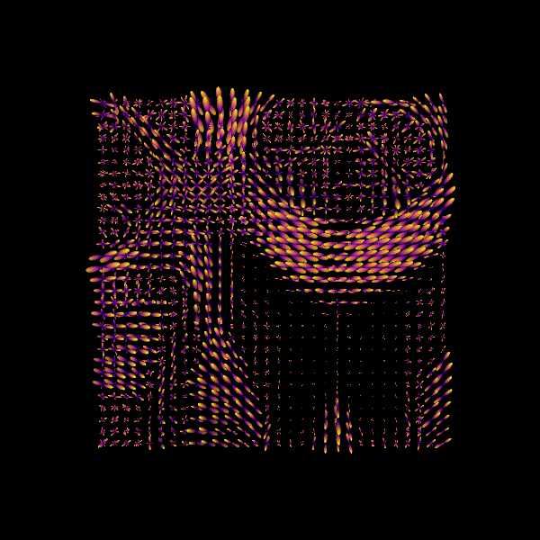
Saving the illustration as csd_odfs.png
Fiber ODFs (fODFs) reconstructed using Constrained Spherical Deconvolution (CSD). For simplicity, we will refer to them just as ODFs.
Step 2. Bingham fitting and Metrics#
Now that we have some ODFs, let us fit the Bingham functions to them by using the function sf_to_bingham:
# A maximum search angle of 45 degrees is chosen arbitrarily for fitting
# each ODF lobe.
max_search_angle = 45
BinghamMetrics = sf_to_bingham(csd_odf, sphere, max_search_angle)
The above function outputs a BinghamMetrics class instance, containing the parameters of the fitted Bingham functions. The metrics of interest contained in the BinghamMetrics class instance are:
- amplitude_lobe (the maximum value for each lobe. Also known as Bingham’s
f_0 parameter.)
- fd_lobe (fiber densitiy: as defined in [1],
one for each peak.)
- fs_lobe (fiber spread: as defined in [1],
one for each peak.)
fd_voxel (voxel fiber density: average of fd across all ODF lobes.)
fs_voxel (voxel fiber spread: average of fs across all ODF lobes.)
- odi2_lobe (orientation dispersion index along Bingham’s second dispersion
axis, one for each lobe.)
- odi_total_lobe (orientation dispersion index averaged across both Binghams’
dispersion axes. Defined in [5].)
- odi1_voxel (orientation dispersion index along Bingham’s first dispersion
axis, averaged across all lobes)
- odi2_voxel (orientation dispersion index along Bingham’s second dispersion
axis, averaged across all lobes)
- odi_total_voxel (orientation dispersion index averaged across both
Binghams’ axes, averaged across all lobes)
- peak_dirs (peak directions in Cartesian coordinates given by the Bingham
fitting, also known as parameter mu_0. These directions are slightly different than the peak directions given by the function peaks_from_model.)
For illustration purposes, the fitted Bingham derived metrics can be visualized using the following lines of code:
bim_odf = BinghamMetrics.odf(sphere)

scene.rm(fodf_spheres)

fodf_spheres = actor.odf_slicer(
    bim_odf, sphere=sphere, scale=0.9, norm=False, colormap="plasma"
)
scene.add(fodf_spheres)

print("Saving the illustration as Bingham_odfs.png")
window.record(scene=scene, out_path="Bingham_odfs.png", size=(600, 600))
if interactive:
    window.show(scene)
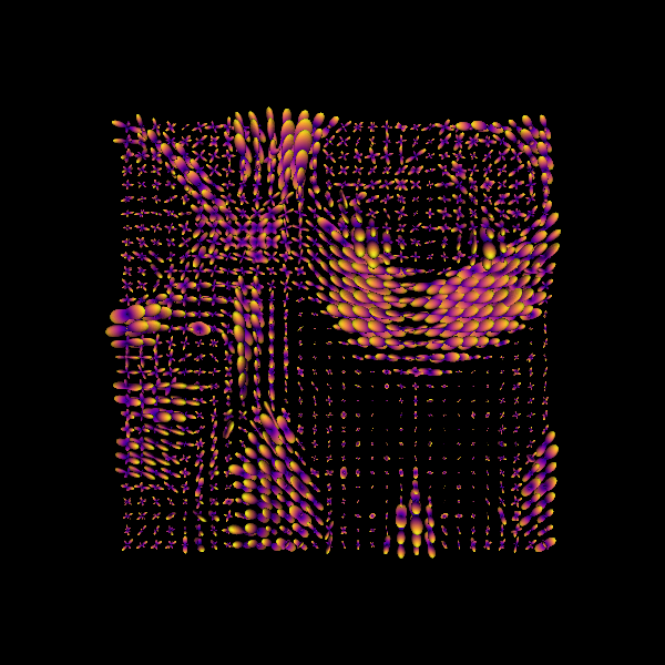
Saving the illustration as Bingham_odfs.png
Bingham functions fitted to CSD fiber ODFs.
Alternatively to fitting Bingham functions to sampled ODFs, DIPY also contains the function sh_to_bingham to perform Bingham fitting from the ODF’s spherical harmonic representation. Although this process may require longer processing times, this function may be useful to avoid memory issues in handling heavily sampled ODFs. For example, you may have reconstructed ODFs using another script and saved their spherical harmonics to disk. This function is for such cases. Below we show the lines of code to use the function sh_to_bingham (feel free to skip these lines if the function sf_to_bingham worked fine for you). Note, to use sh_to_bingham you need to specify the maximum order of spherical harmonics that you defined when reconstructing the ODF. In this example this was set to 8 for the function csd_model:
sh_coeff = csd_fit.shm_coeff
BinghamMetrics = sh_to_bingham(sh_coeff, sphere, max_search_angle)
Step 3. Bingham Metrics#
As mentioned above, reconstructed Bingham functions can be useful to quantify properties from ODFs [1], [2]. Below we plot the Bingham metrics expected to be proportional to the fiber density (FD) of specific fiber populations.
FD_ODF_l1 = BinghamMetrics.fd_lobe[:, :, 0, 0]
FD_ODF_l2 = BinghamMetrics.fd_lobe[:, :, 0, 1]
FD_voxel = BinghamMetrics.fd_voxel[:, :, 0]

FD_images = [FD_ODF_l1[:, -1:1:-1].T, FD_ODF_l2[:, -1:1:-1].T, FD_voxel[:, -1:1:-1].T]
FD_labels = ["FD ODF lobe 1", "FD ODF lobe 2", "FD ODF voxel"]
kwargs = [{"vmin": 0, "vmax": 2}, {"vmin": 0, "vmax": 2}, {"vmin": 0, "vmax": 2}]

print("Saving the illustration as Bingham_fd.png")
image_mosaic(
    FD_images,
    ax_labels=FD_labels,
    ax_kwargs=kwargs,
    figsize=(16, 4),
    filename="Bingham_fd.png",
)

Saving the illustration as Bingham_fd.png

(<Figure size 1600x400 with 6 Axes>, array([<Axes: title={'center': 'FD ODF lobe 1'}>,
       <Axes: title={'center': 'FD ODF lobe 2'}>,
       <Axes: title={'center': 'FD ODF voxel'}>], dtype=object))
The figure shows from left to right: 1) the FD estimated for the first ODF peak (showing larger values in white matter); 2) the FD estimated for the second ODF peak (showing non-zero values in regions of crossing white matter fibers); and 3) the sum of FD estimates across all ODF lobes (quantity that should be proportional to the density of all fibers within each voxel).
Bingham functions can also be used to quantify fiber dispersion from the ODFs [2]. In addition to quantifying a combined orientation dispersion index (ODI_total) for each ODF lobe [5], Bingham functions allow the quantification of dispersion along two main axes (ODI_1 and ODI_2), offering unique information of fiber orientation variability within the brain tissue. Below we show how to extract these indexes from the largest ODF peak. Note, for better visualization of ODI estimates, voxels with total FD lower than 0.5 are masked.
ODIt = BinghamMetrics.odi_total_lobe[:, :, 0, 0]
ODI1 = BinghamMetrics.odi1_lobe[:, :, 0, 0]
ODI2 = BinghamMetrics.odi2_lobe[:, :, 0, 0]

ODIt[FD_voxel < 0.5] = 0
ODI1[FD_voxel < 0.5] = 0
ODI2[FD_voxel < 0.5] = 0

ODI_images = [ODI1[:, -1:1:-1].T, ODI2[:, -1:1:-1].T, ODIt[:, -1:1:-1].T]
ODI_labels = ["ODI_1 (lobe 1)", "ODI_2 (lobe 1)", "ODI_total (lobe 1)"]
kwargs = [{"vmin": 0, "vmax": 0.2}, {"vmin": 0, "vmax": 0.2}, {"vmin": 0, "vmax": 0.2}]
print("Saving the illustration as Bingham_ODI_lobe1.png")
image_mosaic(
    ODI_images,
    ax_labels=ODI_labels,
    ax_kwargs=kwargs,
    figsize=(15, 5),
    filename="Bingham_ODI_lobe1.png",
)
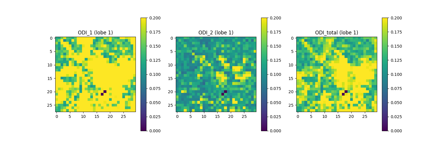
Saving the illustration as Bingham_ODI_lobe1.png

(<Figure size 1500x500 with 6 Axes>, array([<Axes: title={'center': 'ODI_1 (lobe 1)'}>,
       <Axes: title={'center': 'ODI_2 (lobe 1)'}>,
       <Axes: title={'center': 'ODI_total (lobe 1)'}>], dtype=object))
The figure shows from left to right: 1) ODI of the largest ODF lobe along the axis with greater dispersion, a.k.a. ODI_1 (direction in which fibers exhibit the most variability in orientation); 2) ODI of the largest ODF lobe along the axis with lesser dispersion, a.k.a ODI_2 (directions in which fiber orientations are more uniform); and 3) total ODI of the largest lobe across both axes.
Above, we focused on the largest ODF’s lobe, representing the most pronounced fiber population within a voxel. However, this methodology is not limited to a singular lobe since it can be applied to the other ODF lobes. Below, we show the analogous figures for the second-largest ODF lobe. Note that for this figure, regions of white matter that contain only a single fiber population display ODI estimates of zero, corresponding to ODF profiles lacking a second ODF lobe.
ODIt = BinghamMetrics.odi_total_lobe[:, :, 0, 1]
ODI1 = BinghamMetrics.odi1_lobe[:, :, 0, 1]
ODI2 = BinghamMetrics.odi2_lobe[:, :, 0, 1]

ODIt[FD_voxel < 0.5] = 0
ODI1[FD_voxel < 0.5] = 0
ODI2[FD_voxel < 0.5] = 0

ODI_images = [ODI1[:, -1:1:-1].T, ODI2[:, -1:1:-1].T, ODIt[:, -1:1:-1].T]
ODI_labels = ["ODI_1 (lobe 2)", "ODI_2 (lobe 2)", "ODI_voxel (lobe 2)"]
kwargs = [{"vmin": 0, "vmax": 0.2}, {"vmin": 0, "vmax": 0.2}, {"vmin": 0, "vmax": 0.2}]
print("Saving the illustration as Bingham_ODI_lobe2.png")
image_mosaic(
    ODI_images,
    ax_labels=ODI_labels,
    ax_kwargs=kwargs,
    figsize=(15, 5),
    filename="Bingham_ODI_lobe2.png",
)
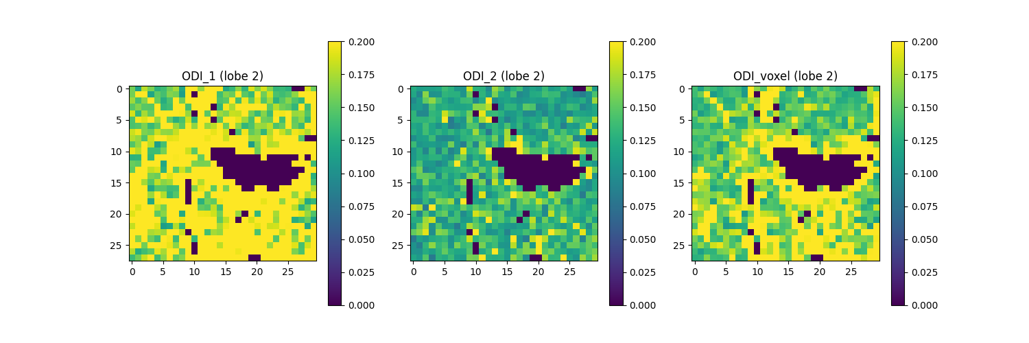
Saving the illustration as Bingham_ODI_lobe2.png

(<Figure size 1500x500 with 6 Axes>, array([<Axes: title={'center': 'ODI_1 (lobe 2)'}>,
       <Axes: title={'center': 'ODI_2 (lobe 2)'}>,
       <Axes: title={'center': 'ODI_voxel (lobe 2)'}>], dtype=object))
The figure shows from left to right: 1) ODI for the second-largest ODF lobe along the axis with greater dispersion a.k.a. ODI_1 (direction in which fibers exhibit the most variability in orientation); 2) ODI for the second-largest ODF lobe along the axis with lesser dispersion a.k.a. ODI_2 (directions in which fiber orientations are more uniform); and 3) total ODI for the second-largest ODF lobe across both axes. In this figure, regions of the white matter that contain only a single fiber population (one ODF lobe) display ODI estimates of zero, corresponding to ODF profiles lacking a second ODF lobe.
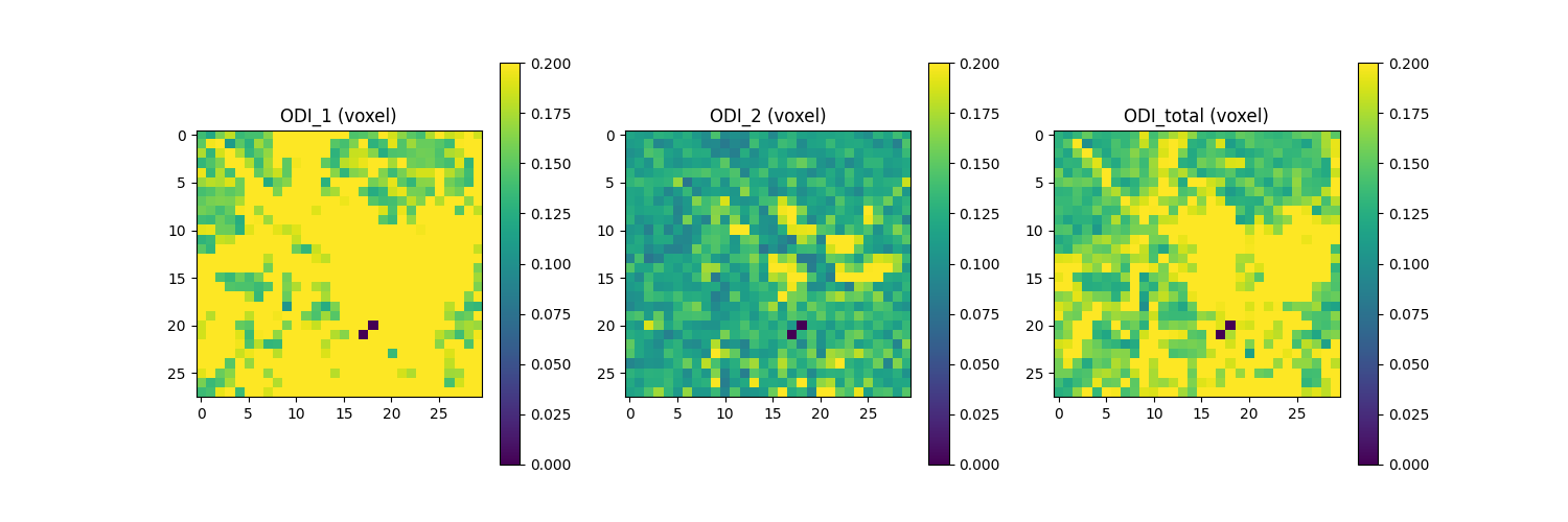
BinghamMetrics can also be used to compute the average ODI quantities across all ODF lobes a.k.a. voxel ODI (see below). The average quantitaties are computed by weigthing each ODF lobe with their respective fiber density (FD) value. These quantities are plotted in the following figure.
ODIt = BinghamMetrics.odi_total_voxel[:, :, 0]
ODI1 = BinghamMetrics.odi1_voxel[:, :, 0]
ODI2 = BinghamMetrics.odi2_voxel[:, :, 0]

ODIt[FD_voxel < 0.5] = 0
ODI1[FD_voxel < 0.5] = 0
ODI2[FD_voxel < 0.5] = 0

ODI_images = [ODI1[:, -1:1:-1].T, ODI2[:, -1:1:-1].T, ODIt[:, -1:1:-1].T]
ODI_labels = ["ODI_1 (voxel)", "ODI_2 (voxel)", "ODI_total (voxel)"]
kwargs = [{"vmin": 0, "vmax": 0.2}, {"vmin": 0, "vmax": 0.2}, {"vmin": 0, "vmax": 0.2}]
print("Saving the illustration as Bingham_ODI.png")
image_mosaic(
    ODI_images,
    ax_labels=ODI_labels,
    ax_kwargs=kwargs,
    figsize=(15, 5),
    filename="Bingham_ODI_voxel.png",
)
Saving the illustration as Bingham_ODI.png

(<Figure size 1500x500 with 6 Axes>, array([<Axes: title={'center': 'ODI_1 (voxel)'}>,
       <Axes: title={'center': 'ODI_2 (voxel)'}>,
       <Axes: title={'center': 'ODI_total (voxel)'}>], dtype=object))
The figure shows from left to right: 1) weighted-averaged ODI_1 across all ODF lobes; 2) weighted-averaged ODI_2 across all ODF lobe; 3) weighted-averaged ODI_total across all ODF lobes.
References#
Total running time of the script: (2 minutes 23.210 seconds)