Using the free water elimination model to remove DTI free water contamination#

As shown previously (see Reconstruction of the diffusion signal with the Tensor model), the diffusion tensor model is a simple way to characterize diffusion anisotropy. However, in regions near the ventricles and parenchyma, anisotropy can be underestimated by partial volume effects of the cerebral spinal fluid (CSF). This free water contamination can particularly corrupt Diffusion Tensor Imaging analysis of microstructural changes when different groups of subjects show different brain morphology (e.g. brain ventricle enlargement associated with brain tissue atrophy that occurs in several brain pathologies and aging).

A way to remove this free water influences is to expand the DTI model to take into account an extra compartment representing the contributions of free water diffusion [Pasternak2009]. The expression of the expanded DTI model is shown below:

\[S(\mathbf{g}, b) = S_0(1-f)e^{-b\mathbf{g}^T \mathbf{D} \mathbf{g}}+S_0fe^{-b D_{iso}}\]

where \(\mathbf{g}\) and \(b\) are diffusion gradient direction and weighted (more information see Reconstruction of the diffusion signal with the Tensor model), \(S(\mathbf{g}, b)\) is thebdiffusion-weighted signal measured, \(S_0\) is the signal in a measurement with no diffusion weighting, \(\mathbf{D}\) is the diffusion tensor, \(f\) the volume fraction of the free water component, and \(D_{iso}\) is the isotropic value of the free water diffusion (normally set to \(3.0 imes 10^{-3} mm^{2}s^{-1}\)).

In this example, we show how to process a diffusion weighting dataset using an adapted version of the free water elimination proposed by [Hoy2014].

The full details of Dipy’s free water DTI implementation was published in [Henriques2017]. Please cite this work if you use this algorithm.

Let’s start by importing the relevant modules:

import numpy as np
import dipy.reconst.fwdti as fwdti
import dipy.reconst.dti as dti
import matplotlib.pyplot as plt
from dipy.data import fetch_hbn
import os.path as op
import nibabel as nib
from dipy.core.gradients import gradient_table

Without spatial constrains the free water elimination model cannot be solved in data acquired from one non-zero b-value [Hoy2014]. Therefore, here we download a dataset that was acquired with multiple b-values.

data_path = fetch_hbn(["NDARAA948VFH"])[1]
dwi_path = op.join(
       data_path, "derivatives", "qsiprep", "sub-NDARAA948VFH",
       "ses-HBNsiteRU", "dwi")

img = nib.load(op.join(
       dwi_path,
       "sub-NDARAA948VFH_ses-HBNsiteRU_acq-64dir_space-T1w_desc-preproc_dwi.nii.gz"))

gtab = gradient_table(
       op.join(dwi_path,
"sub-NDARAA948VFH_ses-HBNsiteRU_acq-64dir_space-T1w_desc-preproc_dwi.bval"),
       op.join(dwi_path,
"sub-NDARAA948VFH_ses-HBNsiteRU_acq-64dir_space-T1w_desc-preproc_dwi.bvec"))

data = np.asarray(img.dataobj)

The free water DTI model can take some minutes to process the full data set. Thus, we use a brain mask that was calculated during pre-processing, to remove the background of the image and avoid unnecessary calculations.

mask_img = nib.load(
       op.join(dwi_path,
"sub-NDARAA948VFH_ses-HBNsiteRU_acq-64dir_space-T1w_desc-brain_mask.nii.gz"))

Moreover, for illustration purposes we process only one slice of the data.

mask = mask_img.get_fdata()

data_small = data[:, :, 50:51]
mask_small = mask[:, :, 50:51]

The free water elimination model fit can then be initialized by instantiating a FreeWaterTensorModel class object:

The data can then be fitted using the fit function of the defined model object:

fwdtifit = fwdtimodel.fit(data_small, mask=mask_small)
  0%|                                                                                                                                        | 0/5148.0 [00:00<?, ?it/s]
  1%|█▋                                                                                                                            | 68/5148.0 [00:00<00:07, 677.65it/s]
  3%|███▍                                                                                                                         | 139/5148.0 [00:00<00:07, 695.42it/s]
  4%|█████                                                                                                                        | 209/5148.0 [00:00<00:07, 668.65it/s]
  5%|██████▋                                                                                                                      | 276/5148.0 [00:00<00:07, 653.19it/s]
  7%|████████▍                                                                                                                    | 347/5148.0 [00:00<00:07, 669.89it/s]
  8%|██████████                                                                                                                   | 415/5148.0 [00:00<00:07, 672.43it/s]
  9%|███████████▊                                                                                                                 | 489/5148.0 [00:00<00:06, 691.99it/s]
 11%|█████████████▌                                                                                                               | 559/5148.0 [00:00<00:06, 693.53it/s]
 12%|███████████████▎                                                                                                             | 632/5148.0 [00:00<00:06, 704.26it/s]
 14%|█████████████████                                                                                                            | 703/5148.0 [00:01<00:06, 702.69it/s]
 15%|██████████████████▊                                                                                                          | 777/5148.0 [00:01<00:06, 711.26it/s]
 17%|████████████████████▋                                                                                                        | 851/5148.0 [00:01<00:05, 718.77it/s]
 18%|██████████████████████▍                                                                                                      | 923/5148.0 [00:01<00:05, 718.35it/s]
 19%|████████████████████████▏                                                                                                    | 995/5148.0 [00:01<00:05, 713.80it/s]
 21%|█████████████████████████▋                                                                                                  | 1067/5148.0 [00:01<00:05, 704.53it/s]
 22%|███████████████████████████▍                                                                                                | 1138/5148.0 [00:01<00:05, 703.31it/s]
 23%|█████████████████████████████                                                                                               | 1209/5148.0 [00:01<00:05, 694.24it/s]C:\Users\skoudoro\AppData\Local\Continuum\Anaconda3\envs\py310\lib\site-packages\scipy\optimize\_minpack_py.py:492: RuntimeWarning: Number of calls to function has reached maxfev = 1800.
  warnings.warn(errors[info][0], RuntimeWarning)

 25%|██████████████████████████████▊                                                                                             | 1279/5148.0 [00:01<00:06, 588.03it/s]
 26%|████████████████████████████████▎                                                                                           | 1341/5148.0 [00:02<00:06, 571.62it/s]
 27%|█████████████████████████████████▋                                                                                          | 1401/5148.0 [00:02<00:06, 563.70it/s]
 29%|███████████████████████████████████▍                                                                                        | 1473/5148.0 [00:02<00:06, 603.49it/s]
 30%|█████████████████████████████████████▏                                                                                      | 1543/5148.0 [00:02<00:05, 628.47it/s]
 31%|██████████████████████████████████████▉                                                                                     | 1614/5148.0 [00:02<00:05, 651.31it/s]
 33%|████████████████████████████████████████▍                                                                                   | 1681/5148.0 [00:02<00:05, 653.90it/s]
 34%|██████████████████████████████████████████▏                                                                                 | 1752/5148.0 [00:02<00:05, 669.52it/s]
 35%|███████████████████████████████████████████▊                                                                                | 1820/5148.0 [00:02<00:05, 629.17it/s]
 37%|█████████████████████████████████████████████▌                                                                              | 1891/5148.0 [00:02<00:05, 650.09it/s]
 38%|███████████████████████████████████████████████▎                                                                            | 1963/5148.0 [00:02<00:04, 669.24it/s]
 40%|█████████████████████████████████████████████████                                                                           | 2036/5148.0 [00:03<00:04, 686.10it/s]
 41%|██████████████████████████████████████████████████▊                                                                         | 2108/5148.0 [00:03<00:04, 695.52it/s]
 42%|████████████████████████████████████████████████████▍                                                                       | 2178/5148.0 [00:03<00:04, 692.09it/s]
 44%|██████████████████████████████████████████████████████▏                                                                     | 2252/5148.0 [00:03<00:04, 703.52it/s]
 45%|███████████████████████████████████████████████████████▉                                                                    | 2323/5148.0 [00:03<00:04, 696.18it/s]
 46%|█████████████████████████████████████████████████████████▋                                                                  | 2393/5148.0 [00:03<00:03, 696.56it/s]
 48%|███████████████████████████████████████████████████████████▎                                                                | 2463/5148.0 [00:03<00:03, 693.63it/s]
 49%|█████████████████████████████████████████████████████████████                                                               | 2533/5148.0 [00:03<00:03, 680.71it/s]
 51%|██████████████████████████████████████████████████████████████▋                                                             | 2602/5148.0 [00:03<00:04, 574.80it/s]
 52%|████████████████████████████████████████████████████████████████▏                                                           | 2663/5148.0 [00:04<00:04, 528.16it/s]
 53%|█████████████████████████████████████████████████████████████████▋                                                          | 2729/5148.0 [00:04<00:04, 560.76it/s]
 54%|███████████████████████████████████████████████████████████████████▏                                                        | 2788/5148.0 [00:04<00:04, 559.37it/s]
 56%|████████████████████████████████████████████████████████████████████▉                                                       | 2861/5148.0 [00:04<00:03, 603.27it/s]
 57%|██████████████████████████████████████████████████████████████████████▍                                                     | 2923/5148.0 [00:04<00:03, 607.20it/s]
 58%|████████████████████████████████████████████████████████████████████████                                                    | 2991/5148.0 [00:04<00:03, 627.26it/s]
 59%|█████████████████████████████████████████████████████████████████████████▌                                                  | 3056/5148.0 [00:04<00:03, 630.21it/s]
 61%|███████████████████████████████████████████████████████████████████████████▏                                                | 3124/5148.0 [00:04<00:03, 644.13it/s]
 62%|████████████████████████████████████████████████████████████████████████████▊                                               | 3189/5148.0 [00:04<00:03, 643.27it/s]
 63%|██████████████████████████████████████████████████████████████████████████████▍                                             | 3257/5148.0 [00:04<00:02, 653.28it/s]
 65%|████████████████████████████████████████████████████████████████████████████████                                            | 3325/5148.0 [00:05<00:02, 658.17it/s]
 66%|█████████████████████████████████████████████████████████████████████████████████▊                                          | 3396/5148.0 [00:05<00:02, 672.68it/s]
 67%|███████████████████████████████████████████████████████████████████████████████████▍                                        | 3466/5148.0 [00:05<00:02, 680.10it/s]
 69%|█████████████████████████████████████████████████████████████████████████████████████▏                                      | 3535/5148.0 [00:05<00:02, 680.71it/s]
 70%|██████████████████████████████████████████████████████████████████████████████████████▊                                     | 3604/5148.0 [00:05<00:02, 666.90it/s]
 71%|████████████████████████████████████████████████████████████████████████████████████████▍                                   | 3671/5148.0 [00:05<00:02, 667.16it/s]
 73%|██████████████████████████████████████████████████████████████████████████████████████████                                  | 3738/5148.0 [00:05<00:02, 617.72it/s]
 74%|███████████████████████████████████████████████████████████████████████████████████████████▌                                | 3801/5148.0 [00:05<00:02, 587.36it/s]
 75%|█████████████████████████████████████████████████████████████████████████████████████████████▏                              | 3871/5148.0 [00:05<00:02, 584.63it/s]
 77%|██████████████████████████████████████████████████████████████████████████████████████████████▉                             | 3944/5148.0 [00:06<00:01, 623.24it/s]
 78%|████████████████████████████████████████████████████████████████████████████████████████████████▌                           | 4008/5148.0 [00:06<00:01, 600.57it/s]
 79%|██████████████████████████████████████████████████████████████████████████████████████████████████▏                         | 4074/5148.0 [00:06<00:01, 616.11it/s]
 80%|███████████████████████████████████████████████████████████████████████████████████████████████████▊                        | 4142/5148.0 [00:06<00:01, 632.65it/s]
 82%|█████████████████████████████████████████████████████████████████████████████████████████████████████▍                      | 4213/5148.0 [00:06<00:01, 653.05it/s]
 83%|███████████████████████████████████████████████████████████████████████████████████████████████████████▏                    | 4282/5148.0 [00:06<00:01, 662.99it/s]
 85%|████████████████████████████████████████████████████████████████████████████████████████████████████████▊                   | 4352/5148.0 [00:06<00:01, 671.86it/s]
 86%|██████████████████████████████████████████████████████████████████████████████████████████████████████████▌                 | 4425/5148.0 [00:06<00:01, 688.08it/s]
 87%|████████████████████████████████████████████████████████████████████████████████████████████████████████████▎               | 4497/5148.0 [00:06<00:00, 694.74it/s]
 89%|██████████████████████████████████████████████████████████████████████████████████████████████████████████████              | 4570/5148.0 [00:06<00:00, 704.21it/s]
 90%|███████████████████████████████████████████████████████████████████████████████████████████████████████████████▊            | 4643/5148.0 [00:07<00:00, 711.15it/s]
 92%|█████████████████████████████████████████████████████████████████████████████████████████████████████████████████▌          | 4715/5148.0 [00:07<00:00, 700.16it/s]
 93%|███████████████████████████████████████████████████████████████████████████████████████████████████████████████████▎        | 4786/5148.0 [00:07<00:00, 695.11it/s]
 94%|████████████████████████████████████████████████████████████████████████████████████████████████████████████████████▉       | 4856/5148.0 [00:07<00:00, 691.70it/s]
 96%|██████████████████████████████████████████████████████████████████████████████████████████████████████████████████████▋     | 4926/5148.0 [00:07<00:00, 687.51it/s]
 97%|████████████████████████████████████████████████████████████████████████████████████████████████████████████████████████▎   | 4995/5148.0 [00:07<00:00, 687.32it/s]
 98%|██████████████████████████████████████████████████████████████████████████████████████████████████████████████████████████  | 5069/5148.0 [00:07<00:00, 701.67it/s]
100%|███████████████████████████████████████████████████████████████████████████████████████████████████████████████████████████▊| 5140/5148.0 [00:07<00:00, 683.19it/s]
100%|████████████████████████████████████████████████████████████████████████████████████████████████████████████████████████████| 5148/5148.0 [00:07<00:00, 656.39it/s]

This 2-steps procedure will create a FreeWaterTensorFit object which contains all the diffusion tensor statistics free for free water contamination. Below we extract the fractional anisotropy (FA) and the mean diffusivity (MD) of the free water diffusion tensor.

FA = fwdtifit.fa
MD = fwdtifit.md

For comparison we also compute the same standard measures processed by the standard DTI model

dtimodel = dti.TensorModel(gtab)

dtifit = dtimodel.fit(data_small, mask=mask_small)

dti_FA = dtifit.fa
dti_MD = dtifit.md

Below the FA values for both free water elimination DTI model and standard DTI model are plotted in panels A and B, while the respective MD values are plotted in panels D and E. For a better visualization of the effect of the free water correction, the differences between these two metrics are shown in panels C and E. In addition to the standard diffusion statistics, the estimated volume fraction of the free water contamination is shown on panel G.

fig1, ax = plt.subplots(2, 4, figsize=(12, 6),
                        subplot_kw={'xticks': [], 'yticks': []})

fig1.subplots_adjust(hspace=0.3, wspace=0.05)
ax.flat[0].imshow(FA[:, :, 0].T, origin='lower',
                  cmap='gray', vmin=0, vmax=1)
ax.flat[0].set_title('A) fwDTI FA')
ax.flat[1].imshow(dti_FA[:, :, 0].T, origin='lower',
                  cmap='gray', vmin=0, vmax=1)
ax.flat[1].set_title('B) standard DTI FA')

FAdiff = abs(FA[:, :, 0] - dti_FA[:, :, 0])
ax.flat[2].imshow(FAdiff.T, cmap='gray', origin='lower', vmin=0, vmax=1)
ax.flat[2].set_title('C) FA difference')

ax.flat[3].axis('off')

ax.flat[4].imshow(MD[:, :, 0].T, origin='lower',
                  cmap='gray', vmin=0, vmax=2.5e-3)
ax.flat[4].set_title('D) fwDTI MD')
ax.flat[5].imshow(dti_MD[:, :, 0].T, origin='lower',
                  cmap='gray', vmin=0, vmax=2.5e-3)
ax.flat[5].set_title('E) standard DTI MD')

MDdiff = abs(MD[:, :, 0] - dti_MD[:, :, 0])
ax.flat[6].imshow(MDdiff.T, origin='lower', cmap='gray', vmin=0, vmax=2.5e-3)
ax.flat[6].set_title('F) MD difference')

F = fwdtifit.f

ax.flat[7].imshow(F[:, :, 0].T, origin='lower',
                  cmap='gray', vmin=0, vmax=1)
ax.flat[7].set_title('G) free water volume')

plt.show()
fig1.savefig('In_vivo_free_water_DTI_and_standard_DTI_measures.png')
reconst fwdti

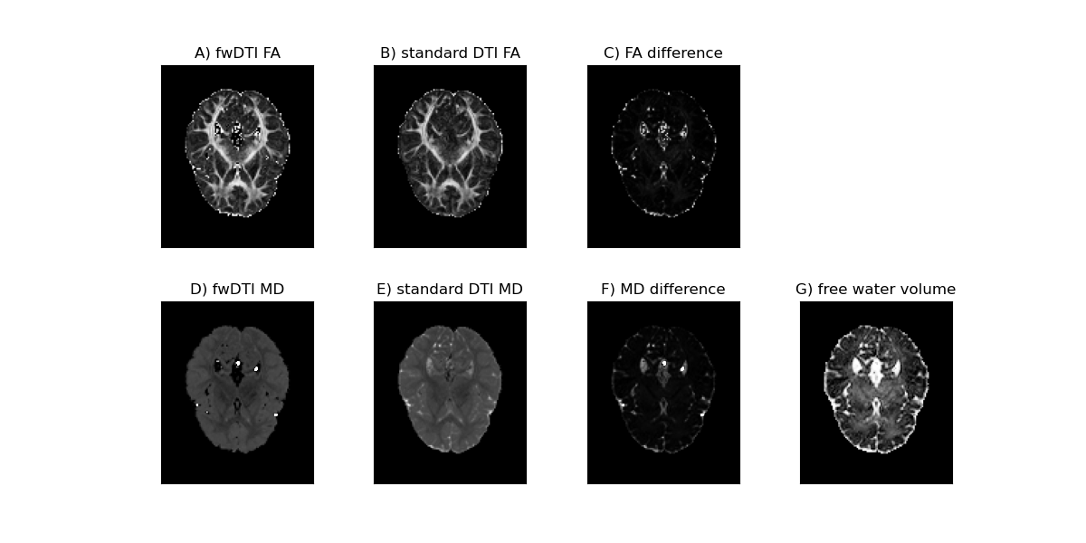
In vivo diffusion measures obtain from the free water DTI and standard DTI. The values of Fractional Anisotropy for the free water DTI model and standard DTI model and their difference are shown in the upper panels (A-C), while respective MD values are shown in the lower panels (D-F). In addition the free water volume fraction estimated from the fwDTI model is shown in panel G.

From the figure, one can observe that the free water elimination model produces in general higher values of FA and lower values of MD than the standard DTI model. These differences in FA and MD estimation are expected due to the suppression of the free water isotropic diffusion components. Unexpected high amplitudes of FA are however observed in the periventricular gray matter. This is a known artefact of regions associated to voxels with high water volume fraction (i.e. voxels containing basically CSF). We are able to remove this problematic voxels by excluding all FA values associated with measured volume fractions above a reasonable threshold of 0.7:

FA[F > 0.7] = 0
dti_FA[F > 0.7] = 0

Above we reproduce the plots of the in vivo FA from the two DTI fits and where we can see that the inflated FA values were practically removed:

fig1, ax = plt.subplots(1, 3, figsize=(9, 3),
                        subplot_kw={'xticks': [], 'yticks': []})

fig1.subplots_adjust(hspace=0.3, wspace=0.05)
ax.flat[0].imshow(FA[:, :, 0].T, origin='lower',
                  cmap='gray', vmin=0, vmax=1)
ax.flat[0].set_title('A) fwDTI FA')
ax.flat[1].imshow(dti_FA[:, :, 0].T, origin='lower',
                  cmap='gray', vmin=0, vmax=1)
ax.flat[1].set_title('B) standard DTI FA')

FAdiff = abs(FA[:, :, 0] - dti_FA[:, :, 0])
ax.flat[2].imshow(FAdiff.T, cmap='gray', origin='lower', vmin=0, vmax=1)
ax.flat[2].set_title('C) FA difference')

plt.show()
fig1.savefig('In_vivo_free_water_DTI_and_standard_DTI_corrected.png')
reconst fwdti

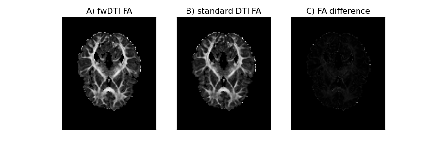
In vivo FA measures obtain from the free water DTI (A) and standard DTI (B) and their difference (C). Problematic inflated FA values of the images were removed by dismissing voxels above a volume fraction threshold of 0.7.

References#

[Pasternak2009]

Pasternak, O., Sochen, N., Gur, Y., Intrator, N., Assaf, Y., 2009. Free water elimination and mapping from diffusion MRI. Magn. Reson. Med. 62(3): 717-30. doi: 10.1002/mrm.22055.

[Hoy2014] (1,2)

Hoy, A.R., Koay, C.G., Kecskemeti, S.R., Alexander, A.L., 2014. Optimization of a free water elimination two-compartmental model for diffusion tensor imaging. NeuroImage 103, 323-333. doi: 10.1016/j.neuroimage.2014.09.053

[Henriques2017]

Henriques, R.N., Rokem, A., Garyfallidis, E., St-Jean, S., Peterson E.T., Correia, M.M., 2017. [Re] Optimization of a free water elimination two-compartment model for diffusion tensor imaging. ReScience volume 3, issue 1, article number 2

Total running time of the script: (0 minutes 11.914 seconds)

Gallery generated by Sphinx-Gallery