Denoise images using Adaptive Soft Coefficient Matching (ASCM)

The adaptive soft coefficient matching (ASCM) as described in [Coupe11] is a improved extension of non-local means (NLMEANS) denoising. ASCM gives a better denoised images from two standard non-local means denoised versions of the original data with different degrees sharpness. Here, one denoised input is more “smooth” than the other (the easiest way to achieve this denoising is use non_local_means with two different patch radii).

ASCM involves these basic steps

• Computes wavelet decomposition of the noisy as well as denoised inputs

• Combines the wavelets for the output image in a way that it takes it’s smoothness (low frequency components) from the input with larger smoothing, and the sharp features (high frequency components) from the input with less smoothing.

This way ASCM gives us a well denoised output while preserving the sharpness of the image features.

Let us load the necessary modules

import numpy as np
import matplotlib.pyplot as plt
from dipy.core.gradients import gradient_table
from dipy.data import get_fnames
from dipy.denoise.noise_estimate import estimate_sigma
from dipy.io.image import load_nifti, save_nifti
from dipy.io.gradients import read_bvals_bvecs
from time import time
from dipy.denoise.non_local_means import non_local_means
from dipy.denoise.adaptive_soft_matching import adaptive_soft_matching

Choose one of the data from the datasets in dipy

dwi_fname, dwi_bval_fname, dwi_bvec_fname = get_fnames('sherbrooke_3shell')
data, affine = load_nifti(dwi_fname)
bvals, bvecs = read_bvals_bvecs(dwi_bval_fname, dwi_bvec_fname)
gtab = gradient_table(bvals, bvecs)

mask = data[..., 0] > 80
data = data[..., 1]

print("vol size", data.shape)

t = time()

vol size (128, 128, 60)

In order to generate the two pre-denoised versions of the data we will use the non_local_means denoining # noqa E501 For non_local_means first we need to estimate the standard deviation of the noise. We use N=4 since the Sherbrooke dataset was acquired on a 1.5T Siemens scanner with a 4 array head coil.

sigma = estimate_sigma(data, N=4)

For the denoised version of the original data which preserves sharper features, we perform non-local means with smaller patch size.

den_small = non_local_means(
    data,
    sigma=sigma,
    mask=mask,
    patch_radius=1,
    block_radius=1,
    rician=True)

For the denoised version of the original data that implies more smoothing, we perform non-local means with larger patch size.

den_large = non_local_means(
    data,
    sigma=sigma,
    mask=mask,
    patch_radius=2,
    block_radius=1,
    rician=True)

Now we perform the adaptive soft coefficient matching. Empirically we set the adaptive parameter in ascm to be the average of the local noise variance, in this case the sigma itself.

den_final = adaptive_soft_matching(data, den_small, den_large, sigma[0])

print("total time", time() - t)

total time 9.760449409484863

To access the quality of this denoising procedure, we plot the an axial slice of the original data, it’s denoised output and residuals.

axial_middle = data.shape[2] // 2

original = data[:, :, axial_middle].T
final_output = den_final[:, :, axial_middle].T
difference = np.abs(final_output.astype(np.float64) - original.astype(np.float64))
difference[~mask[:, :, axial_middle].T] = 0

fig, ax = plt.subplots(1, 3)
ax[0].imshow(original, cmap='gray', origin='lower')
ax[0].set_title('Original')
ax[1].imshow(final_output, cmap='gray', origin='lower')
ax[1].set_title('ASCM output')
ax[2].imshow(difference, cmap='gray', origin='lower')
ax[2].set_title('Residual')
for i in range(3):
    ax[i].set_axis_off()

plt.savefig('denoised_ascm.png', bbox_inches='tight')

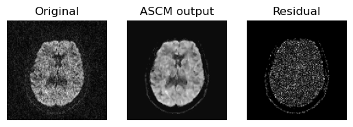
Showing the axial slice without (left) and with (middle) ASCM denoising.

From the above figure we can see that the residual is really uniform in nature which dictates that ASCM denoises the data while preserving the sharpness of the features. Now, we are Saving the entire denoised output in denoised_ascm.nii.gz file.

save_nifti('denoised_ascm.nii.gz', den_final, affine)

For comparison propose we also plot the outputs of the non_local_means (both with the larger as well as with the smaller patch radius) with the ASCM output.

fig, ax = plt.subplots(1, 4)
ax[0].imshow(original, cmap='gray', origin='lower')
ax[0].set_title('Original')
ax[1].imshow(den_small[..., axial_middle].T, cmap='gray', origin='lower',
             interpolation='none')
ax[1].set_title('NLMEANS small')
ax[2].imshow(den_large[..., axial_middle].T, cmap='gray', origin='lower',
             interpolation='none')
ax[2].set_title('NLMEANS large')
ax[3].imshow(final_output, cmap='gray', origin='lower', interpolation='none')
ax[3].set_title('ASCM ')
for i in range(4):
    ax[i].set_axis_off()

plt.savefig('ascm_comparison.png', bbox_inches='tight')

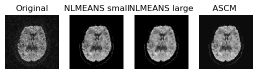
Comparing outputs of the NLMEANS and ASCM.

From the above figure, we can observe that the information of two pre-denoised versions of the raw data, ASCM outperforms standard non-local means in suppressing noise and preserving feature sharpness.

References

[Coupe11]

Pierrick Coupe, Jose Manjon, Montserrat Robles, Louis Collins. Adaptive Multiresolution Non-Local Means Filter for 3D MR Image Denoising. IET Image Processing, Institution of Engineering and Technology, 2011. <00645538>