Calculate DSI-based scalar maps

We show how to calculate two DSI-based scalar maps: return to origin probability (RTOP) [1] and mean square displacement (MSD) [2], [3] on your dataset.

First import the necessary modules:

import matplotlib.pyplot as plt
import numpy as np

from dipy.core.gradients import gradient_table
from dipy.data import get_fnames
from dipy.io.gradients import read_bvals_bvecs
from dipy.io.image import load_nifti
from dipy.reconst.dsi import DiffusionSpectrumModel

Download and get the data filenames for this tutorial.

fraw, fbval, fbvec = get_fnames(name="taiwan_ntu_dsi")

img contains a nibabel Nifti1Image object (data) and gtab contains a GradientTable object (gradient information e.g. b-values). For example to read the b-values it is possible to write print(gtab.bvals).

Load the raw diffusion data and the affine.

data, affine = load_nifti(fraw)
bvals, bvecs = read_bvals_bvecs(fbval, fbvec)
bvecs[1:] = bvecs[1:] / np.sqrt(np.sum(bvecs[1:] * bvecs[1:], axis=1))[:, None]
gtab = gradient_table(bvals, bvecs=bvecs)

print(f"data.shape {data.shape}")

data.shape (96, 96, 60, 203)

Instantiate the Model and apply it to the data.

dsmodel = DiffusionSpectrumModel(gtab, qgrid_size=35, filter_width=18.5)

Let’s just use one slice only from the data.

dataslice = data[30:70, 20:80, data.shape[2] // 2]

Normalize the signal by the b0

dataslice = dataslice / (dataslice[..., 0, None]).astype(float)

Calculate the return to origin probability on the signal that corresponds to the integral of the signal.

print("Calculating... rtop_signal")
rtop_signal = dsmodel.fit(dataslice).rtop_signal()

Calculating... rtop_signal

Now we calculate the return to origin probability on the propagator, that corresponds to its central value. By default the propagator is divided by its sum in order to obtain a properly normalized pdf, however this normalization changes the values of RTOP, therefore in order to compare it with the RTOP previously calculated on the signal we turn the normalized parameter to false.

print("Calculating... rtop_pdf")
rtop_pdf = dsmodel.fit(dataslice).rtop_pdf(normalized=False)

Calculating... rtop_pdf

In theory, these two measures must be equal, to show that we calculate the mean square error on this two measures.

mse = np.sum((rtop_signal - rtop_pdf) ** 2) / rtop_signal.size
print(f"mse = {mse:f}")

mse = 0.000000

Leaving the normalized parameter to the default changes the values of the RTOP but not the contrast between the voxels.

print("Calculating... rtop_pdf_norm")
rtop_pdf_norm = dsmodel.fit(dataslice).rtop_pdf()

Calculating... rtop_pdf_norm

Let’s calculate the mean square displacement on the normalized propagator.

print("Calculating... msd_norm")
msd_norm = dsmodel.fit(dataslice).msd_discrete()

Calculating... msd_norm

Turning the normalized parameter to false makes it possible to calculate the mean square displacement on the propagator without normalization.

print("Calculating... msd")
msd = dsmodel.fit(dataslice).msd_discrete(normalized=False)

Calculating... msd

Show the RTOP images and save them in rtop.png.

fig = plt.figure(figsize=(6, 6))
ax1 = fig.add_subplot(2, 2, 1, title="rtop_signal")
ax1.set_axis_off()
ind = ax1.imshow(rtop_signal.T, interpolation="nearest", origin="lower")
plt.colorbar(ind)
ax2 = fig.add_subplot(2, 2, 2, title="rtop_pdf_norm")
ax2.set_axis_off()
ind = ax2.imshow(rtop_pdf_norm.T, interpolation="nearest", origin="lower")
plt.colorbar(ind)
ax3 = fig.add_subplot(2, 2, 3, title="rtop_pdf")
ax3.set_axis_off()
ind = ax3.imshow(rtop_pdf.T, interpolation="nearest", origin="lower")
plt.colorbar(ind)
plt.savefig("rtop.png")

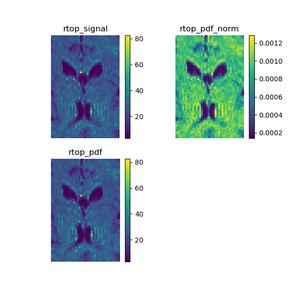
Return to origin probability.

Show the MSD images and save them in msd.png.

fig = plt.figure(figsize=(7, 3))
ax1 = fig.add_subplot(1, 2, 1, title="msd_norm")
ax1.set_axis_off()
ind = ax1.imshow(msd_norm.T, interpolation="nearest", origin="lower")
plt.colorbar(ind)
ax2 = fig.add_subplot(1, 2, 2, title="msd")
ax2.set_axis_off()
ind = ax2.imshow(msd.T, interpolation="nearest", origin="lower")
plt.colorbar(ind)
plt.savefig("msd.png")

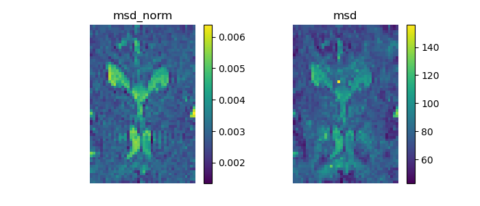
Mean square displacement.

References

[1]

Maxime Descoteaux, Rachid Deriche, Denis Le Bihan, Jean-François Mangin, and Cyril Poupon. Multiple q-shell diffusion propagator imaging. Medical Image Analysis, 15(4):603–621, 2011. Special section on IPMI 2009. URL: https://doi.org/10.1016/j.media.2010.07.001, doi:10.1016/j.media.2010.07.001.

[2]

Yu-Chien Wu and Andrew L. Alexander. Hybrid diffusion imaging. NeuroImage, 36(3):617–629, 2007. URL: https://doi.org/10.1016/j.neuroimage.2007.02.050, doi:10.1016/j.neuroimage.2007.02.050.

[3]

Yu-Chien Wu, Aaron S. Field, and Andrew L. Alexander. Computation of Diffusion Function Measures in $q$-Space Using Magnetic Resonance Hybrid Diffusion Imaging. IEEE Transactions on Medical Imaging, 27(6):858–865, 2008. doi:10.1109/TMI.2008.922696.