Streamline length and size reduction

This example shows how to calculate the lengths of a set of streamlines and also how to compress the streamlines without considerably reducing their lengths or overall shape.

A streamline in DIPY is represented as a numpy array of size \((N imes 3)\) where each row of the array represents a 3D point of the streamline. A set of streamlines is represented with a list of numpy arrays of size \((N_i imes 3)\) for \(i=1:M\) where \(M\) is the number of streamlines in the set.

import matplotlib.pyplot as plt
import numpy as np

from dipy.tracking.distances import approx_polygon_track
from dipy.tracking.streamline import set_number_of_points
from dipy.tracking.utils import length
from dipy.viz import actor, window

Let’s first create a simple simulation of a bundle of streamlines using a cosine function.

def simulated_bundles(no_streamlines=50, n_pts=100):
    rng = np.random.default_rng()

    t = np.linspace(-10, 10, n_pts)

    bundle = []
    for i in np.linspace(3, 5, no_streamlines):
        pts = np.vstack((np.cos(2 * t / np.pi), np.zeros(t.shape) + i, t)).T
        bundle.append(pts)

    start = rng.integers(10, 30, no_streamlines)
    end = rng.integers(60, 100, no_streamlines)

    bundle = [
        10 * streamline[start[i] : end[i]] for (i, streamline) in enumerate(bundle)
    ]
    bundle = [np.ascontiguousarray(streamline) for streamline in bundle]

    return bundle


bundle = simulated_bundles()

print(f"This bundle has {len(bundle)} streamlines")

This bundle has 50 streamlines

Using the length function we can retrieve the lengths of each streamline. Below we show the histogram of the lengths of the streamlines.

lengths = list(length(bundle))

fig_hist, ax = plt.subplots(1)
ax.hist(lengths, color="burlywood")
ax.set_xlabel("Length")
ax.set_ylabel("Count")
# plt.show()
plt.legend()
plt.savefig("length_histogram.png")

/Users/skoudoro/devel/dipy/doc/examples_revamped/streamline_analysis/streamline_length.py:66: UserWarning: No artists with labels found to put in legend.  Note that artists whose label start with an underscore are ignored when legend() is called with no argument.
  plt.legend()

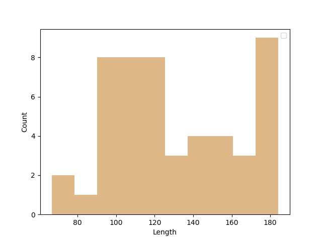
Histogram of lengths of the streamlines

Length will return the length in the units of the coordinate system that streamlines are currently. So, if the streamlines are in world coordinates then the lengths will be in millimeters (mm). If the streamlines are for example in native image coordinates of voxel size 2mm isotropic then you will need to multiply the lengths by 2 if you want them to correspond to mm. In this example we process simulated data without units, however this information is good to have in mind when you calculate lengths with real data.

Next, let’s find the number of points that each streamline has.

n_pts = [len(streamline) for streamline in bundle]

Often, streamlines are represented with more points than what is actually necessary for specific applications. Also, sometimes every streamline has a different number of points, which could be a problem for some algorithms. The function set_number_of_points can be used to set the number of points of a streamline at a specific number and at the same time enforce that all the segments of the streamline will have equal length.

bundle_downsampled = set_number_of_points(bundle, nb_points=12)
n_pts_ds = [len(s) for s in bundle_downsampled]

Alternatively, the function approx_polygon_track allows reducing the number of points so that there are more points in curvy regions and less points in less curvy regions. In contrast with set_number_of_points it does not enforce that segments should be of equal size.

bundle_downsampled2 = [approx_polygon_track(s, 0.25) for s in bundle]
n_pts_ds2 = [len(streamline) for streamline in bundle_downsampled2]

Both, set_number_of_points and approx_polygon_track can be thought as methods for lossy compression of streamlines.

# Enables/disables interactive visualization
interactive = False

scene = window.Scene()
scene.SetBackground(*window.colors.white)
bundle_actor = actor.streamtube(bundle, colors=window.colors.red, linewidth=0.3)

scene.add(bundle_actor)

bundle_actor2 = actor.streamtube(
    bundle_downsampled, colors=window.colors.red, linewidth=0.3
)
bundle_actor2.SetPosition(0, 40, 0)

bundle_actor3 = actor.streamtube(
    bundle_downsampled2, colors=window.colors.red, linewidth=0.3
)
bundle_actor3.SetPosition(0, 80, 0)

scene.add(bundle_actor2)
scene.add(bundle_actor3)

scene.set_camera(position=(0, 0, 0), focal_point=(30, 0, 0))
window.record(scene=scene, out_path="simulated_cosine_bundle.png", size=(900, 900))
if interactive:
    window.show(scene)

Initial bundle (down), downsampled at 12 equidistant points (middle), downsampled with points that are not equidistant (up).

From the figure above we can see that all 3 bundles look quite similar. However, when we plot the histogram of the number of points used for each streamline, it becomes obvious that we have managed to reduce in a great amount the size of the initial dataset.

fig_hist, ax = plt.subplots(1)
ax.hist(n_pts, color="r", histtype="step", label="initial")
ax.hist(n_pts_ds, color="g", histtype="step", label="set_number_of_points (12)")
ax.hist(n_pts_ds2, color="b", histtype="step", label="approx_polygon_track (0.25)")
ax.set_xlabel("Number of points")
ax.set_ylabel("Count")

# plt.show()
plt.legend()
plt.savefig("n_pts_histogram.png")

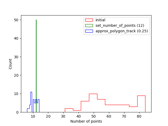
Histogram of the number of points of the streamlines.

Finally, we can also show that the lengths of the streamlines haven’t changed considerably after applying the two methods of downsampling.

lengths_downsampled = list(length(bundle_downsampled))
lengths_downsampled2 = list(length(bundle_downsampled2))

fig, ax = plt.subplots(1)
ax.plot(lengths, color="r", label="initial")
ax.plot(lengths_downsampled, color="g", label="set_number_of_points (12)")
ax.plot(lengths_downsampled2, color="b", label="approx_polygon_track (0.25)")
ax.set_xlabel("Streamline ID")
ax.set_ylabel("Length")

# plt.show()
plt.legend()
plt.savefig("lengths_plots.png")

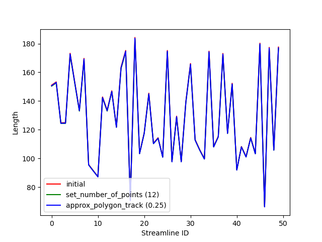
Lengths of each streamline for every one of the 3 bundles.