Linear fascicle evaluation (LiFE)

Evaluating the results of tractography algorithms is one of the biggest challenges for diffusion MRI. One proposal for evaluation of tractography results is to use a forward model that predicts the signal from each of a set of streamlines, and then fit a linear model to these simultaneous predictions [1].

We will use streamlines generated using probabilistic tracking on CSA peaks. For brevity, we will include in this example only streamlines going through the corpus callosum connecting left to right superior frontal cortex. The process of tracking and finding these streamlines is fully demonstrated in the Connectivity Matrices, ROI Intersections and Density Maps example. If this example has been run, we can read the streamlines from file. Otherwise, we’ll run that example first, by importing it. This provides us with all of the variables that were created in that example:

from os.path import join as pjoin

import matplotlib
import matplotlib.pyplot as plt
from mpl_toolkits.axes_grid1 import AxesGrid
import numpy as np

# We'll need to know where the corpus callosum is from these variables:
from dipy.core.gradients import gradient_table
import dipy.core.optimize as opt
from dipy.data import fetch_stanford_tracks, get_fnames
from dipy.io.gradients import read_bvals_bvecs
from dipy.io.image import load_nifti, load_nifti_data
from dipy.io.streamline import load_trk
import dipy.tracking.life as life
from dipy.viz import actor, colormap as cmap, window

hardi_fname, hardi_bval_fname, hardi_bvec_fname = get_fnames(name="stanford_hardi")
label_fname = get_fnames(name="stanford_labels")
t1_fname = get_fnames(name="stanford_t1")

data, affine, hardi_img = load_nifti(hardi_fname, return_img=True)
labels = load_nifti_data(label_fname)
t1_data = load_nifti_data(t1_fname)
bvals, bvecs = read_bvals_bvecs(hardi_bval_fname, hardi_bvec_fname)
gtab = gradient_table(bvals, bvecs=bvecs)

cc_slice = labels == 2

# Let's now fetch a set of streamlines from the Stanford HARDI dataset.
# Those streamlines were generated during the
# :ref:`sphx_glr_examples_built_streamline_analysis_streamline_tools.py` example.
# Read the candidates from file in voxel space:

streamlines_files = fetch_stanford_tracks()
lr_superiorfrontal_path = pjoin(streamlines_files[1], "hardi-lr-superiorfrontal.trk")

candidate_sl_sft = load_trk(lr_superiorfrontal_path, "same")
candidate_sl_sft.to_vox()
candidate_sl = candidate_sl_sft.streamlines

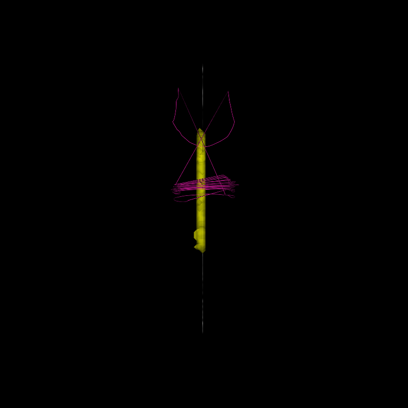
The streamlines that are entered into the model are termed ‘candidate streamlines’ (or a ‘candidate connectome’):

Let’s visualize the initial candidate group of streamlines in 3D, relative to the anatomical structure of this brain:

# Enables/disables interactive visualization
interactive = False

candidate_streamlines_actor = actor.streamtube(
    candidate_sl, colors=cmap.line_colors(candidate_sl)
)
cc_ROI_actor = actor.contour_from_roi(cc_slice, color=(1.0, 1.0, 0.0), opacity=0.5)

vol_actor = actor.slicer(t1_data)

vol_actor.display(x=40)
vol_actor2 = vol_actor.copy()
vol_actor2.display(z=35)

# Add display objects to canvas
scene = window.Scene()
scene.add(candidate_streamlines_actor)
scene.add(cc_ROI_actor)
scene.add(vol_actor)
scene.add(vol_actor2)
window.record(scene=scene, n_frames=1, out_path="life_candidates.png", size=(800, 800))
if interactive:
    window.show(scene)

Candidate connectome before life optimization

Next, we initialize a LiFE model. We import the dipy.tracking.life module, which contains the classes and functions that implement the model:

fiber_model = life.FiberModel(gtab)

Since we read the streamlines from a file, already in the voxel space, we do not need to transform them into this space. Otherwise, if the streamline coordinates were in the world space (relative to the scanner iso-center, or relative to the mid-point of the AC-PC-connecting line), we would use this:

inv_affine = np.linalg.inv(hardi_img.affine)

the inverse transformation from world space to the voxel space as the affine for the following model fit.

The next step is to fit the model, producing a FiberFit class instance, that stores the data, as well as the results of the fitting procedure.

The LiFE model posits that the signal in the diffusion MRI volume can be explained by the streamlines, by the equation

\[y = X\beta\]

Where \(y\) is the diffusion MRI signal, \(\beta\) are a set of weights on the streamlines and \(X\) is a design matrix. This matrix has the dimensions \(m\) by \(n\), where \(m=n_{voxels} \cdot n_{directions}\), and \(n_{voxels}\) is the set of voxels in the ROI that contains the streamlines considered in this model. The \(i^{th}\) column of the matrix contains the expected contributions of the \(i^{th}\) streamline (arbitrarily ordered) to each of the voxels. \(X\) is a sparse matrix, because each streamline traverses only a small percentage of the voxels. The expected contributions of the streamline are calculated using a forward model, where each node of the streamline is modeled as a cylindrical fiber compartment with Gaussian diffusion, using the diffusion tensor model. See [1] for more detail on the model, and variations of this model.

fiber_fit = fiber_model.fit(data, candidate_sl, affine=np.eye(4))

The FiberFit class instance holds various properties of the model fit. For example, it has the weights \(\beta\), that are assigned to each streamline. In most cases, a tractography through some region will include redundant streamlines, and these streamlines will have \(\beta_i\) that are 0.

fig, ax = plt.subplots(1)
ax.hist(fiber_fit.beta, bins=100, histtype="step")
ax.set_xlabel("Fiber weights")
ax.set_ylabel("# fibers")
fig.savefig("beta_histogram.png")

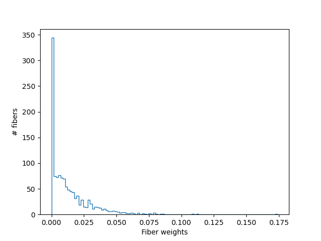
LiFE streamline weights

We use \(\beta\) to filter out these redundant streamlines, and generate an optimized group of streamlines:

optimized_sl = [np.vstack(candidate_sl)[np.where(fiber_fit.beta > 0)[0]]]
scene = window.Scene()
scene.add(actor.streamtube(optimized_sl, colors=cmap.line_colors(optimized_sl)))
scene.add(cc_ROI_actor)
scene.add(vol_actor)
window.record(scene=scene, n_frames=1, out_path="life_optimized.png", size=(800, 800))
if interactive:
    window.show(scene)

Streamlines selected via LiFE optimization

The new set of streamlines should do well in fitting the data, and redundant streamlines have presumably been removed (in this case, about 50% of the streamlines).

But how well does the model do in explaining the diffusion data? We can quantify that: the FiberFit class instance has a predict method, which can be used to invert the model and predict back either the data that was used to fit the model, or other unseen data (e.g. in cross-validation, see K-fold cross-validation for model comparison).

Without arguments, the .predict() method will predict the diffusion signal for the same gradient table that was used in the fit data, but gtab and S0 keyword arguments can be used to predict for other acquisition schemes and other baseline non-diffusion-weighted signals.

model_predict = fiber_fit.predict()

We will focus on the error in prediction of the diffusion-weighted data, and calculate the root of the mean squared error.

model_error = model_predict - fiber_fit.data
model_rmse = np.sqrt(np.mean(model_error[:, 10:] ** 2, -1))

As a baseline against which we can compare, we calculate another error term. In this case, we assume that the weight for each streamline is equal to zero. This produces the naive prediction of the mean of the signal in each voxel.

beta_baseline = np.zeros(fiber_fit.beta.shape[0])
pred_weighted = np.reshape(
    opt.spdot(fiber_fit.life_matrix, beta_baseline),
    (fiber_fit.vox_coords.shape[0], np.sum(~gtab.b0s_mask)),
)
mean_pred = np.empty((fiber_fit.vox_coords.shape[0], gtab.bvals.shape[0]))
S0 = fiber_fit.b0_signal

Since the fitting is done in the demeaned S/S0 domain, we need to add back the mean and then multiply by S0 in every voxel:

mean_pred[..., gtab.b0s_mask] = S0[:, None]
mean_pred[..., ~gtab.b0s_mask] = (pred_weighted + fiber_fit.mean_signal[:, None]) * S0[
    :, None
]
mean_error = mean_pred - fiber_fit.data
mean_rmse = np.sqrt(np.mean(mean_error**2, -1))

First, we can compare the overall distribution of errors between these two alternative models of the ROI. We show the distribution of differences in error (improvement through model fitting, relative to the baseline model). Here, positive values denote an improvement in error with model fit, relative to without the model fit.

fig, ax = plt.subplots(1)
ax.hist(mean_rmse - model_rmse, bins=100, histtype="step")
ax.text(
    0.2,
    0.9,
    f"Median RMSE, mean model: {np.median(mean_rmse):.2f}",
    horizontalalignment="left",
    verticalalignment="center",
    transform=ax.transAxes,
)
ax.text(
    0.2,
    0.8,
    f"Median RMSE, LiFE: {np.median(model_rmse):.2f}",
    horizontalalignment="left",
    verticalalignment="center",
    transform=ax.transAxes,
)
ax.set_xlabel("RMS Error")
ax.set_ylabel("# voxels")
fig.savefig("error_histograms.png")

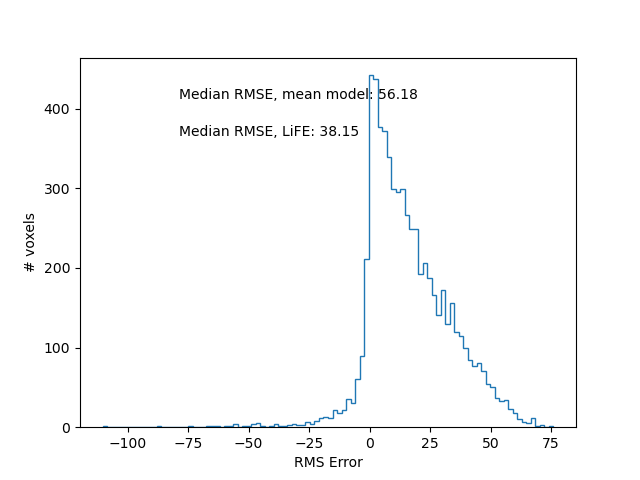
Improvement in error with fitting of the LiFE model.

Second, we can show the spatial distribution of the two error terms, and of the improvement with the model fit:

vol_model = np.ones(data.shape[:3]) * np.nan
vol_model[
    fiber_fit.vox_coords[:, 0], fiber_fit.vox_coords[:, 1], fiber_fit.vox_coords[:, 2]
] = model_rmse
vol_mean = np.ones(data.shape[:3]) * np.nan
vol_mean[
    fiber_fit.vox_coords[:, 0], fiber_fit.vox_coords[:, 1], fiber_fit.vox_coords[:, 2]
] = mean_rmse
vol_improve = np.ones(data.shape[:3]) * np.nan
vol_improve[
    fiber_fit.vox_coords[:, 0], fiber_fit.vox_coords[:, 1], fiber_fit.vox_coords[:, 2]
] = mean_rmse - model_rmse
sl_idx = 49
fig = plt.figure()
fig.subplots_adjust(left=0.05, right=0.95)
ax = AxesGrid(
    fig,
    111,
    nrows_ncols=(1, 3),
    label_mode="1",
    share_all=True,
    cbar_location="top",
    cbar_mode="each",
    cbar_size="10%",
    cbar_pad="5%",
)
ax[0].matshow(np.rot90(t1_data[sl_idx, :, :]), cmap=matplotlib.cm.bone)
im = ax[0].matshow(np.rot90(vol_model[sl_idx, :, :]), cmap=matplotlib.cm.hot)
ax.cbar_axes[0].colorbar(im)
ax[1].matshow(np.rot90(t1_data[sl_idx, :, :]), cmap=matplotlib.cm.bone)
im = ax[1].matshow(np.rot90(vol_mean[sl_idx, :, :]), cmap=matplotlib.cm.hot)
ax.cbar_axes[1].colorbar(im)
ax[2].matshow(np.rot90(t1_data[sl_idx, :, :]), cmap=matplotlib.cm.bone)
im = ax[2].matshow(np.rot90(vol_improve[sl_idx, :, :]), cmap=matplotlib.cm.RdBu)
ax.cbar_axes[2].colorbar(im)
for lax in ax:
    lax.set_xticks([])
    lax.set_yticks([])
fig.savefig("spatial_errors.png")

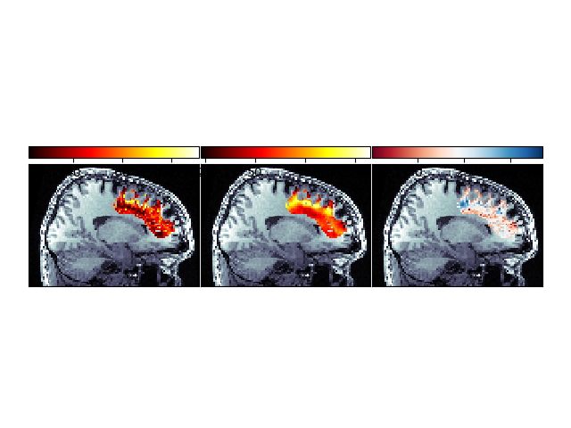
Spatial distribution of error and improvement.

This image demonstrates that in many places, fitting the LiFE model results in substantial reduction of the error.

Note that for full-brain tractographies LiFE can require large amounts of memory. For detailed memory profiling of the algorithm, based on the streamlines generated in An introduction to the Probabilistic Direction Getter, see this IPython notebook.

For the Matlab implementation of LiFE, head over to Franco Pestilli’s github webpage.

References

[1] (1,2)

Franco Pestilli, Jason D. Yeatman, Ariel Rokem, Kendrick N. Kay, and Brian A. Wandell. Evaluation and statistical inference for human connectomes. Nature Methods, 11(10):1058–1063, 2014. URL: https://doi.org/10.1038/nmeth.3098, doi:10.1038/nmeth.3098.