Suppress Gibbs oscillations

Magnetic Resonance (MR) images are reconstructed from the Fourier coefficients of acquired k-space images. Since only a finite number of Fourier coefficients can be acquired in practice, reconstructed MR images can be corrupted by Gibbs artefacts, which is manifested by intensity oscillations adjacent to edges of different tissues types [1]. Although this artefact affects MR images in general, in the context of diffusion-weighted imaging, Gibbs oscillations can be magnified in derived diffusion-based estimates [1], [2].

In the following example, we show how to suppress Gibbs artefacts of MR images. This algorithm is based on an adapted version of a sub-voxel Gibbs suppression procedure [3]. Full details of the implemented algorithm can be found in chapter 3 of [4] (please cite [3], [4] if you are using this code).

The algorithm to suppress Gibbs oscillations can be imported from the denoise module of dipy:

import matplotlib.pyplot as plt
import numpy as np

from dipy.data import get_fnames, read_cenir_multib
from dipy.denoise.gibbs import gibbs_removal
from dipy.io.image import load_nifti_data
import dipy.reconst.msdki as msdki
from dipy.segment.mask import median_otsu

We first apply this algorithm to a T1-weighted dataset which can be fetched using the following code:

t1_fname, t1_denoised_fname, ap_fname = get_fnames(name="tissue_data")
t1 = load_nifti_data(t1_denoised_fname)

Let’s plot a slice of this dataset.

axial_slice = 88
t1_slice = t1[..., axial_slice]

fig = plt.figure(figsize=(15, 4))
fig.subplots_adjust(wspace=0.2)

t1_slice = np.rot90(t1_slice)

plt.subplot(1, 2, 1)
plt.imshow(t1_slice, cmap="gray", vmin=100, vmax=400)
plt.colorbar()
fig.savefig("structural.png")

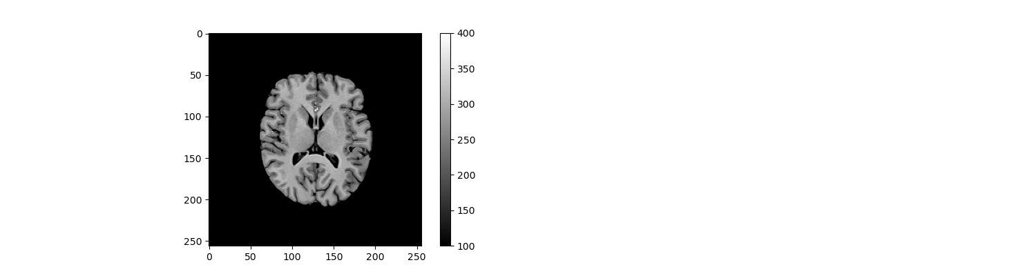
Representative slice of a T1-weighted structural image.

Due to the high quality of the data, Gibbs artefacts are not visually evident in this dataset. Therefore, to analyse the benefits of the Gibbs suppression algorithm, Gibbs artefacts are artificially introduced by removing high frequencies of the image’s Fourier transform.

c = np.fft.fft2(t1_slice)
c = np.fft.fftshift(c)
N = c.shape[0]
c_crop = c[64:192, 64:192]
N = c_crop.shape[0]
t1_gibbs = abs(np.fft.ifft2(c_crop) / 4)

Gibbs oscillation suppression of this single data slice can be performed by running the following command:

t1_unring = gibbs_removal(t1_gibbs, inplace=False)

Let’s plot the results:

fig1, ax = plt.subplots(1, 3, figsize=(12, 6), subplot_kw={"xticks": [], "yticks": []})

ax.flat[0].imshow(t1_gibbs, cmap="gray", vmin=100, vmax=400)
ax.flat[0].annotate(
    "Rings",
    fontsize=10,
    xy=(81, 70),
    color="red",
    xycoords="data",
    xytext=(30, 0),
    textcoords="offset points",
    arrowprops={"arrowstyle": "->", "color": "red"},
)
ax.flat[0].annotate(
    "Rings",
    fontsize=10,
    xy=(75, 50),
    color="red",
    xycoords="data",
    xytext=(30, 0),
    textcoords="offset points",
    arrowprops={"arrowstyle": "->", "color": "red"},
)

ax.flat[1].imshow(t1_unring, cmap="gray", vmin=100, vmax=400)
ax.flat[1].annotate(
    "WM/GM",
    fontsize=10,
    xy=(75, 50),
    color="green",
    xycoords="data",
    xytext=(30, 0),
    textcoords="offset points",
    arrowprops={"arrowstyle": "->", "color": "green"},
)

ax.flat[2].imshow(t1_unring - t1_gibbs, cmap="gray", vmin=0, vmax=10)
ax.flat[2].annotate(
    "Rings",
    fontsize=10,
    xy=(81, 70),
    color="red",
    xycoords="data",
    xytext=(30, 0),
    textcoords="offset points",
    arrowprops={"arrowstyle": "->", "color": "red"},
)
ax.flat[2].annotate(
    "Rings",
    fontsize=10,
    xy=(75, 50),
    color="red",
    xycoords="data",
    xytext=(30, 0),
    textcoords="offset points",
    arrowprops={"arrowstyle": "->", "color": "red"},
)
plt.show()
fig1.savefig("Gibbs_suppression_structural.png")

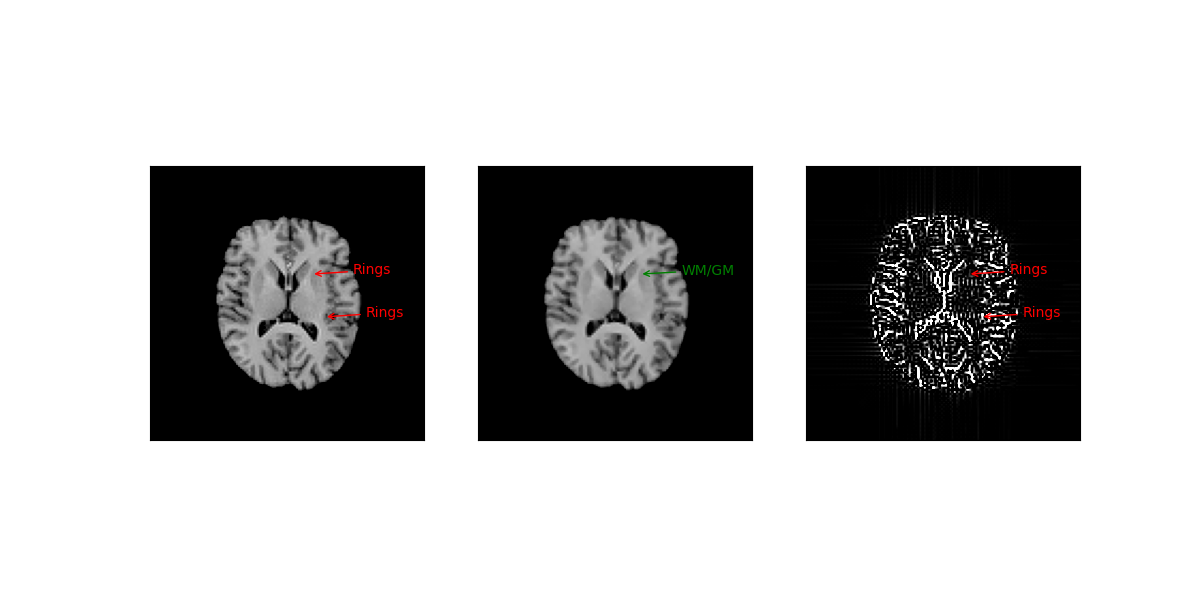
Uncorrected and corrected structural images are shown in the left and middle panels, while the difference between these images is shown in the right panel.

The image artificially corrupted with Gibb’s artefacts is shown in the left panel. In this panel, the characteristic ringing profile of Gibbs artefacts can be visually appreciated (see intensity oscillations pointed by the red arrows). The corrected image is shown in the middle panel. One can appreciate that artefactual oscillations are visually suppressed without compromising the contrast between white and grey matter (e.g. details pointed by the green arrow). The difference between uncorrected and corrected data is plotted in the right panel which highlights the suppressed Gibbs ringing profile.

Now let’s show how to use the Gibbs suppression algorithm in diffusion-weighted images. We fetch the multi-shell diffusion-weighted dataset which was kindly supplied by Romain Valabrègue, CENIR, ICM, Paris [5].

bvals = [200, 400, 1000, 2000]

img, gtab = read_cenir_multib(bvals=bvals)

data = np.asarray(img.dataobj)

For illustration purposes, we select two slices of this dataset

data_slices = data[:, :, 40:42, :]

Gibbs oscillation suppression of all multi-shell data and all slices can be performed in the following way:

data_corrected = gibbs_removal(data_slices, slice_axis=2, num_processes=-1)

Due to the high dimensionality of diffusion-weighted data, we recommend that you specify which is the axis of data matrix that corresponds to different slices in the above step. This is done by using the optional parameter ‘slice_axis’.

Below we plot the results for an image acquired with b-value=0:

fig2, ax = plt.subplots(1, 3, figsize=(12, 6), subplot_kw={"xticks": [], "yticks": []})

ax.flat[0].imshow(
    data_slices[:, :, 0, 0].T, cmap="gray", origin="lower", vmin=0, vmax=10000
)
ax.flat[0].set_title("Uncorrected b0")
ax.flat[1].imshow(
    data_corrected[:, :, 0, 0].T, cmap="gray", origin="lower", vmin=0, vmax=10000
)
ax.flat[1].set_title("Corrected b0")
ax.flat[2].imshow(
    data_corrected[:, :, 0, 0].T - data_slices[:, :, 0, 0].T,
    cmap="gray",
    origin="lower",
    vmin=-500,
    vmax=500,
)
ax.flat[2].set_title("Gibbs residuals")

plt.show()
fig2.savefig("Gibbs_suppression_b0.png")

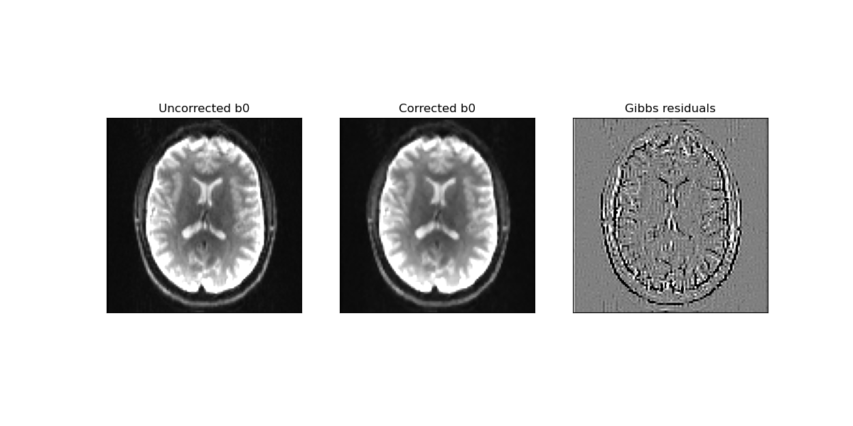
Uncorrected (left panel) and corrected (middle panel) b-value=0 images. For reference, the difference between uncorrected and corrected images is shown in the right panel.

The above figure shows that the benefits of suppressing Gibbs artefacts is hard to observe on b-value=0 data. Therefore, diffusion derived metrics for both uncorrected and corrected data are computed using the mean signal diffusion kurtosis image technique (Mean signal diffusion kurtosis imaging (MSDKI)).

To avoid unnecessary calculations on the background of the image, we also compute a brain mask.

# Create a brain mask
maskdata, mask = median_otsu(
    data_slices,
    vol_idx=range(10, 50),
    median_radius=3,
    numpass=1,
    autocrop=False,
    dilate=1,
)

# Define mean signal diffusion kurtosis model
dki_model = msdki.MeanDiffusionKurtosisModel(gtab)

# Fit the uncorrected data
dki_fit = dki_model.fit(data_slices, mask=mask)
MSKini = dki_fit.msk

# Fit the corrected data
dki_fit = dki_model.fit(data_corrected, mask=mask)
MSKgib = dki_fit.msk

Let’s plot the results

fig3, ax = plt.subplots(1, 3, figsize=(12, 12), subplot_kw={"xticks": [], "yticks": []})

ax.flat[0].imshow(MSKini[:, :, 0].T, cmap="gray", origin="lower", vmin=0, vmax=1.5)
ax.flat[0].set_title("MSK (uncorrected)")
ax.flat[0].annotate(
    "Rings",
    fontsize=12,
    xy=(59, 63),
    color="red",
    xycoords="data",
    xytext=(45, 0),
    textcoords="offset points",
    arrowprops={"arrowstyle": "->", "color": "red"},
)

ax.flat[1].imshow(MSKgib[:, :, 0].T, cmap="gray", origin="lower", vmin=0, vmax=1.5)
ax.flat[1].set_title("MSK (corrected)")

ax.flat[2].imshow(
    MSKgib[:, :, 0].T - MSKini[:, :, 0].T,
    cmap="gray",
    origin="lower",
    vmin=-0.2,
    vmax=0.2,
)
ax.flat[2].set_title("MSK (uncorrected - corrected")
ax.flat[2].annotate(
    "Rings",
    fontsize=12,
    xy=(59, 63),
    color="red",
    xycoords="data",
    xytext=(45, 0),
    textcoords="offset points",
    arrowprops={"arrowstyle": "->", "color": "red"},
)

plt.show()
fig3.savefig("Gibbs_suppression_msdki.png")

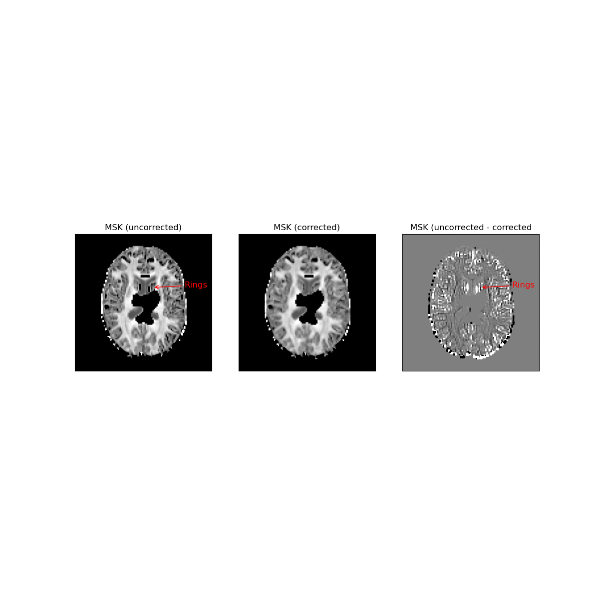
Uncorrected and corrected mean signal kurtosis images are shown in the left and middle panels. The difference between uncorrected and corrected images are show in the right panel.

In the left panel of the figure above, Gibbs artefacts can be appreciated by the negative values of mean signal kurtosis (black voxels) adjacent to the brain ventricle (red arrows). These negative values seem to be suppressed after the gibbs_removal function is applied. For a better visualization of Gibbs oscillations, the difference between corrected and uncorrected images are shown in the right panel.

References

[1] (1,2)

Jelle Veraart, Els Fieremans, Ileana O. Jelescu, Florian Knoll, and Dmitry S. Novikov. Gibbs ringing in diffusion MRI. Magnetic Resonance in Medicine, 76(1):301–314, July 2016. URL: https://doi.org/10.1002/mrm.25866, doi:10.1002/mrm.25866.

[2]

Daniele Perrone, Jan Aelterman, Aleksandra Pižurica, Ben Jeurissen, Wilfried Philips, and Alexander Leemans. The effect of Gibbs ringing artifacts on measures derived from diffusion MRI. NeuroImage, 120:441–455, 2015. URL: https://doi.org/10.1016/j.neuroimage.2015.06.068, doi:10.1016/j.neuroimage.2015.06.068.

[3] (1,2)

Elias Kellner, Bibek Dhital, Valerij G. Kiselev, and Marco Reisert. Gibbs-ringing artifact removal based on local subvoxel-shifts. Magnetic Resonance in Medicine, 76(5):1574–1581, 2016. URL: https://doi.org/10.1002/mrm.26054, doi:10.1002/mrm.26054.

[4] (1,2)

Rafael Neto Henriques. Advanced Methods for Diffusion MRI Data Analysis and their Application to the Healthy Ageing Brain. PhD thesis, Cambridge University, Cambridge, United Kingdom, 2018. URL: https://doi.org/10.17863/CAM.29356, doi:10.17863/CAM.29356.

[5]

Romain Valabrègue. Diffusion MRI measured at multiple b-values. University Libraries, eScience Institute Faculty Research, 2015. doi:http://hdl.handle.net/1773/33311.