Intravoxel incoherent motion (IVIM)

The intravoxel incoherent motion (IVIM) model describes diffusion and perfusion in the signal acquired with a diffusion MRI sequence that contains multiple low b-values. The IVIM model can be understood as an adaptation of the work of Stejskal and Tanner [1] in biological tissue, and was proposed by Le Bihan [2]. The model assumes two compartments: a slow moving compartment, where particles diffuse in a Brownian fashion as a consequence of thermal energy, and a fast moving compartment (the vascular compartment), where blood moves as a consequence of a pressure gradient. In the first compartment, the diffusion coefficient is \(\mathbf{D}\) while in the second compartment, a pseudo diffusion term \(\mathbf{D^*}\) is introduced that describes the displacement of the blood elements in an assumed randomly laid out vascular network, at the macroscopic level. According to [2], \(\mathbf{D^*}\) is greater than \(\mathbf{D}\).

The IVIM model expresses the MRI signal as follows:

\[S(b)=S_0(fe^{-bD^*}+(1-f)e^{-bD})\]

where \(\mathbf{b}\) is the diffusion gradient weighing value (which is dependent on the measurement parameters), \(\mathbf{S_{0}}\) is the signal in the absence of diffusion gradient sensitization, \(\mathbf{f}\) is the perfusion fraction, \(\mathbf{D}\) is the diffusion coefficient and \(\mathbf{D^*}\) is the pseudo-diffusion constant, due to vascular contributions.

In the following example we show how to fit the IVIM model on a diffusion-weighted dataset and visualize the diffusion and pseudo-diffusion coefficients. First, we import all relevant modules:

import matplotlib.pyplot as plt

from dipy.core.gradients import gradient_table
from dipy.data import get_fnames
from dipy.io.gradients import read_bvals_bvecs
from dipy.io.image import load_nifti_data
from dipy.reconst.ivim import IvimModel

We get an IVIM dataset using DIPY’s data fetcher read_ivim. This dataset was acquired with 21 b-values in 3 different directions. Volumes corresponding to different directions were registered to each other, and averaged across directions. Thus, this dataset has 4 dimensions, with the length of the last dimension corresponding to the number of b-values. In order to use this model the data should contain signals measured at 0 bvalue.

fraw, fbval, fbvec = get_fnames(name="ivim")

The gtab contains a GradientTable object (information about the gradients e.g. b-values and b-vectors). We get the data from the file using load_nifti_data.

data = load_nifti_data(fraw)
bvals, bvecs = read_bvals_bvecs(fbval, fbvec)
gtab = gradient_table(bvals, bvecs=bvecs, b0_threshold=0)
print(f"data.shape {data.shape}")

data.shape (256, 256, 54, 21)

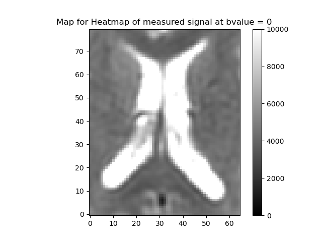
The data has 54 slices, with 256-by-256 voxels in each slice. The fourth dimension corresponds to the b-values in the gtab. Let us visualize the data by taking a slice midway(z=33) at \(\mathbf{b} = 0\).

z = 33
b = 0

plt.imshow(data[:, :, z, b].T, origin="lower", cmap="gray", interpolation="nearest")
plt.axhline(y=100)
plt.axvline(x=170)
plt.savefig("ivim_data_slice.png")
plt.close()

Heat map of a slice of data

The region around the intersection of the cross-hairs in the figure contains cerebral spinal fluid (CSF), so it should have a very high \(\mathbf{f}\) and \(\mathbf{D^*}\), the area just medial to that is white matter so that should be lower, and the region more laterally contains a mixture of gray matter and CSF. That should give us some contrast to see the values varying across the regions.

x1, x2 = 90, 155
y1, y2 = 90, 170
data_slice = data[x1:x2, y1:y2, z, :]

plt.imshow(
    data[x1:x2, y1:y2, z, b].T, origin="lower", cmap="gray", interpolation="nearest"
)
plt.savefig("CSF_slice.png")
plt.close()

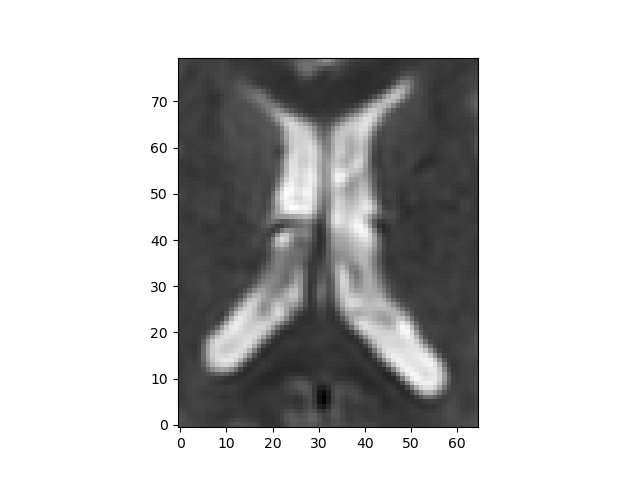
Heat map of the CSF slice selected.

Now that we have prepared the datasets we can go forward with the ivim fit. We provide two methods of fitting the parameters of the IVIM multi-exponential model explained above. We first fit the model with a simple fitting approach by passing the option fit_method=’trr’. This method uses a two-stage approach: first, a linear fit used to get quick initial guesses for the parameters \(\mathbf{S_{0}}\) and \(\mathbf{D}\) by considering b-values greater than split_b_D (default: 400))and assuming a mono-exponential signal. This is based on the assumption that at high b-values the signal can be approximated as a mono exponential decay and by taking the logarithm of the signal values a linear fit can be obtained. Another linear fit for S0 (bvals < split_b_S0 (default: 200)) follows and f is estimated using \(1 - S0_{prime}/S0\). Then a non-linear least-squares fitting is performed to fit D_star and f. If the two_stage flag is set to True while initializing the model, a final non-linear least squares fitting is performed for all the parameters. All initializations for the model such as split_b_D are passed while creating the IvimModel. If you are using Scipy 0.17, you can also set bounds by setting bounds=([0., 0., 0.,0.], [np.inf, 1., 1., 1.])) while initializing the IvimModel.

For brevity, we focus on a small section of the slice as selected above, to fit the IVIM model. First, we instantiate the IvimModel object.

ivimmodel = IvimModel(gtab, fit_method="trr")

/opt/homebrew/Caskroom/miniforge/base/envs/py312-test/lib/python3.12/site-packages/dipy/testing/decorators.py:192: UserWarning: Bounds for this fit have been set from experiments and literature survey. To change the bounds, please input your bounds in model definition...
  return func(*args, **kwargs)

To fit the model, call the fit method and pass the data for fitting.

ivimfit = ivimmodel.fit(data_slice)

/opt/homebrew/Caskroom/miniforge/base/envs/py312-test/lib/python3.12/site-packages/dipy/reconst/ivim.py:332: UserWarning: x0 obtained from linear fitting is not feasible as initial guess for leastsq while estimating f and D_star. Using parameters from the linear fit.
  f, D_star = self.estimate_f_D_star(params_f_D_star, data, S0, D)
/opt/homebrew/Caskroom/miniforge/base/envs/py312-test/lib/python3.12/site-packages/dipy/reconst/ivim.py:336: UserWarning: x0 is unfeasible for leastsq fitting. Returning x0 values from the linear fit.
  params_two_stage = self._leastsq(data, params_linear)
/opt/homebrew/Caskroom/miniforge/base/envs/py312-test/lib/python3.12/site-packages/dipy/reconst/multi_voxel.py:85: UserWarning: Bounds are violated for leastsq fitting. Returning parameters from linear fit
  svf = single_voxel_fit(self, data[ijk], **kwargs)

The fit method creates a IvimFit object which contains the parameters of the model obtained after fitting. These are accessible through the model_params attribute of the IvimFit object. The parameters are arranged as a 4D array, corresponding to the spatial dimensions of the data, and the last dimension (of length 4) corresponding to the model parameters according to the following order : \(\mathbf{S_{0}, f, D^*, D}\).

ivimparams = ivimfit.model_params
print(f"ivimparams.shape : {ivimparams.shape}")

ivimparams.shape : (65, 80, 4)

As we see, we have a 20x20 slice at the height z = 33. Thus we have 400 voxels. We will now plot the parameters obtained from the fit for a voxel and also various maps for the entire slice. This will give us an idea about the diffusion and perfusion in that section. Let(i, j) denote the coordinate of the voxel. We have already fixed the z component as 33 and hence we will get a slice which is 33 units above.

i, j = 10, 10
estimated_params = ivimfit.model_params[i, j, :]
print(estimated_params)

[3.97863113e+03 2.00000000e-01 1.69394175e-03 6.71052306e-04]

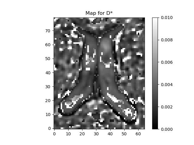
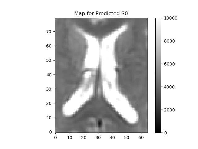
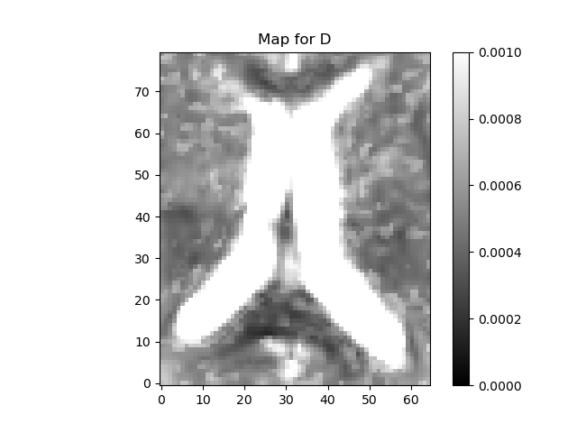
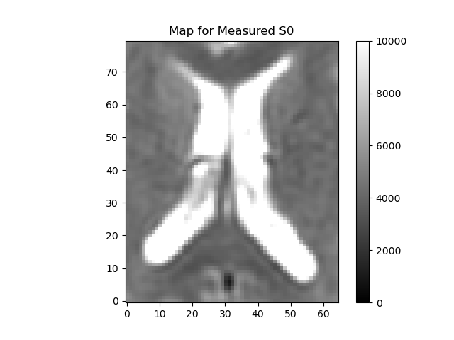
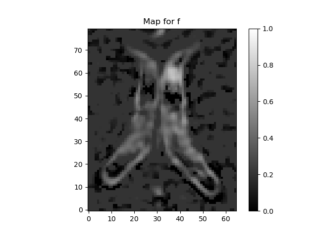
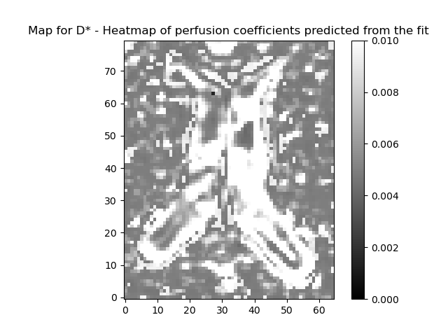
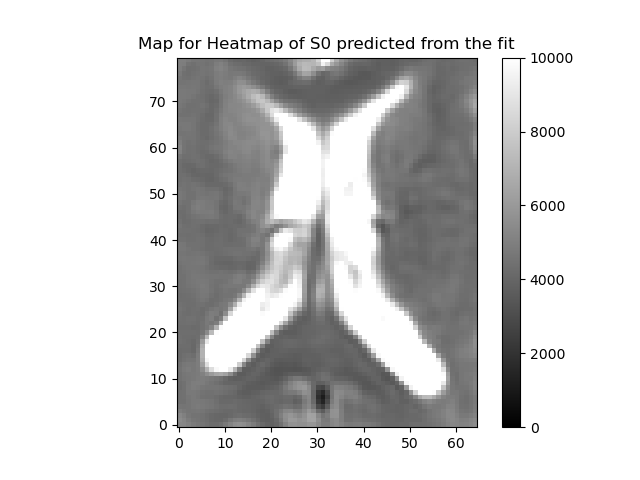
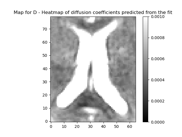
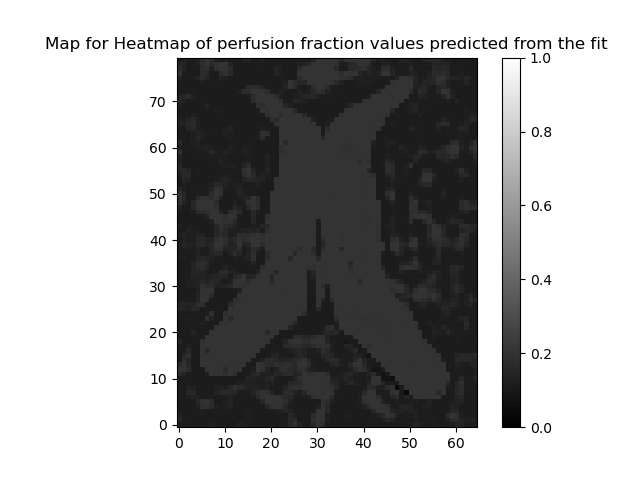
Now we can map the perfusion and diffusion maps for the slice. We will plot a heatmap showing the values using a colormap. It will be useful to define a plotting function for the heatmap here since we will use it to plot for all the IVIM parameters. We will need to specify the lower and upper limits for our data. For example, the perfusion fractions should be in the range (0,1). Similarly, the diffusion and pseudo-diffusion constants are much smaller than 1. We pass an argument called variable to out plotting function which gives the label for the plot.

def plot_map(raw_data, variable, limits, filename):
    fig, ax = plt.subplots(1)
    lower, upper = limits
    ax.set_title(f"Map for {variable}")
    im = ax.imshow(
        raw_data.T,
        origin="lower",
        clim=(lower, upper),
        cmap="gray",
        interpolation="nearest",
    )
    fig.colorbar(im)
    fig.savefig(filename)

Let us get the various plots with fit_method = ‘trr’ so that we can visualize them in one page

plot_map(ivimfit.S0_predicted, "Predicted S0", (0, 10000), "predicted_S0.png")
plot_map(data_slice[:, :, 0], "Measured S0", (0, 10000), "measured_S0.png")
plot_map(ivimfit.perfusion_fraction, "f", (0, 1), "perfusion_fraction.png")
plot_map(ivimfit.D_star, "D*", (0, 0.01), "perfusion_coeff.png")
plot_map(ivimfit.D, "D", (0, 0.001), "diffusion_coeff.png")

• 
• 
• 
• 
• 

Next, we will fit the same model with a more refined optimization process with fit_method=’VarPro’ (for “Variable Projection”). The VarPro computes the IVIM parameters using the MIX approach [3]. This algorithm uses three different optimizers. It starts with a differential evolution algorithm and fits the parameters in the power of exponentials. Then the fitted parameters in the first step are utilized to make a linear convex problem. Using a convex optimization, the volume fractions are determined. The last step is non-linear least-squares fitting on all the parameters. The results of the first and second optimizers are utilized as the initial values for the last step of the algorithm.

As opposed to the ‘trr’ fitting method, this approach does not need to set any thresholds on the bvals to differentiate between the perfusion (pseudo-diffusion) and diffusion portions and fits the parameters simultaneously. Making use of the three step optimization mentioned above increases the convergence basin for fitting the multi-exponential functions of microstructure models. This method has been described in further detail in [4] and [3].

ivimmodel_vp = IvimModel(gtab, fit_method="VarPro")
ivimfit_vp = ivimmodel_vp.fit(data_slice)

Just like the ‘trr’ fit method, ‘VarPro’ creates a IvimFit object which contains the parameters of the model obtained after fitting. These are accessible through the model_params attribute of the IvimFit object. The parameters are arranged as a 4D array, corresponding to the spatial dimensions of the data, and the last dimension (of length 4) corresponding to the model parameters according to the following order : \(\mathbf{S_{0}, f, D^*, D}\).

i, j = 10, 10
estimated_params = ivimfit_vp.model_params[i, j, :]
print(estimated_params)

[4.15609803e+03 1.09732631e-01 9.86662595e-03 7.19170060e-04]

To compare the fit using fit_method=’VarPro’ and fit_method=’trr’, we can plot one voxel’s signal and the model fit using both methods.

We will use the predict method of the IvimFit objects, to get the predicted signal, based on each one of the model fit methods.

fig, ax = plt.subplots(1)

ax.scatter(gtab.bvals, data_slice[i, j, :], color="green", label="Measured signal")

ivim_trr_predict = ivimfit.predict(gtab)[i, j, :]

ax.plot(gtab.bvals, ivim_trr_predict, label="trr prediction")

S0_est, f_est, D_star_est, D_est = ivimfit.model_params[i, j, :]

trr_pro_param_est = (
    f"S0={S0_est:06.3f} f={f_est:06.4f}\n" f"D*={D_star_est:06.5f} D={D_est:06.5f}"
)
text_fit = f"""trr param estimates:\n {trr_pro_param_est}"""

ax.text(
    0.65,
    0.80,
    text_fit,
    horizontalalignment="center",
    verticalalignment="center",
    transform=plt.gca().transAxes,
)

ivim_predict_vp = ivimfit_vp.predict(gtab)[i, j, :]
ax.plot(gtab.bvals, ivim_predict_vp, label="VarPro prediction")

ax.set_xlabel("bvalues")
ax.set_ylabel("Signals")

S0_est, f_est, D_star_est, D_est = ivimfit_vp.model_params[i, j, :]

var_pro_param_est = (
    f"S0={S0_est:06.3f} f={f_est:06.4f}\n" f"D*={D_star_est:06.5f} D={D_est:06.5f}"
)
text_fit = f"""VarPro param estimates:\n{var_pro_param_est}"""

ax.text(
    0.65,
    0.50,
    text_fit,
    horizontalalignment="center",
    verticalalignment="center",
    transform=plt.gca().transAxes,
)

fig.legend(loc="upper right")
fig.savefig("ivim_voxel_plot.png")

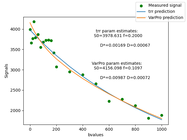
Plot of the signal from one voxel.

Let us get the various plots with fit_method = ‘VarPro’ so that we can visualize them in one page

plt.figure()
plot_map(
    ivimfit_vp.S0_predicted,
    "Heatmap of S0 predicted from the fit",
    (0, 10000),
    "predicted_S0.png",
)
plot_map(
    data_slice[..., 0],
    "Heatmap of measured signal at bvalue = 0",
    (0, 10000),
    "measured_S0.png",
)
plot_map(
    ivimfit_vp.perfusion_fraction,
    "Heatmap of perfusion fraction values predicted from the fit",
    (0, 1),
    "perfusion_fraction.png",
)
plot_map(
    ivimfit_vp.D_star,
    "D* - Heatmap of perfusion coefficients predicted from the fit",
    (0, 0.01),
    "perfusion_coeff.png",
)
plot_map(
    ivimfit_vp.D,
    "D - Heatmap of diffusion coefficients predicted from the fit",
    (0, 0.001),
    "diffusion_coeff.png",
)

• 
• 
• 
• 
• 

References

[1]

Edward O. Stejskal and John E. Tanner. Spin Diffusion Measurements: Spin Echoes in the Presence of a Time-Dependent Field Gradient. The Journal of Chemical Physics, 42(1):288–292, January 1965. doi:http://dx.doi.org/10.1063/1.1695690.

[2] (1,2)

Denis Le Bihan, Eric Breton, Denis Lallemand, M. L. Aubin, Jacqueline Vignaud, and Maurice Laval-Jeantet. Separation of diffusion and perfusion in intravoxel incoherent motion MR imaging. Radiology, 168(2):497–505, 1988. URL: https://doi.org/10.1148/radiology.168.2.3393671, doi:10.1148/radiology.168.2.3393671.

[3] (1,2)

Hamza Farooq, Junqian Xu, Jung Who Nam, Daniel F. Keefe, Essa Yacoub, Tryphon Georgiou, and Christophe Lenglet. Microstructure imaging of crossing (mix) white matter fibers from diffusion mri. Scientific Reports, 6(1):38927, December 2016. URL: https://doi.org/10.1038/srep38927, doi:10.1038/srep38927.

[4]

Shreyas Fadnavis, Marco Reisert, Hamza Farooq, Maryam Afzali, Cheng Hu, Bago Amirbekian, and Eleftherios Garyfallidis. MicroLearn: Framework for machine learning, reconstruction, optimization and microstructure modeling. In ISMRM 27th Annual Meeting & Exhibition SMRT 28th Annual Meeting. Montréal, Canada, 2019. International Society for Magnetic Resonance in Medicine (ISMRM).