Reconstruction of the diffusion signal with the kurtosis tensor model (DKI)

Diffusional Kurtosis Imaging (DKI) is an expansion of the Diffusion Tensor Imaging (DTI) model (see Reconstruction of the diffusion signal with DTI (single tensor) model). In addition to the Diffusion Tensor (DT), DKI quantifies the degree to which water diffusion in biological tissues is non-Gaussian using the Kurtosis Tensor (KT) [1].

Measurements of non-Gaussian diffusion from DKI are of interest because they were shown to provide extra information about microstructural alterations in both health and disease (for a review see our paper [2]). Moreover, in contrast to DTI, DKI can provide metrics of tissue microscopic heterogeneity that are less sensitive to confounding effects in the orientation of tissue components, thus providing better characterization in general white matter configurations (including regions of fibers crossing, fanning, and/or dispersing) and gray matter [3], [2]. Although DKI aims primarily to quantify the degree of non-Gaussian diffusion without establishing concrete biophysical assumptions, DKI can also be related to microstructural models to infer specific biophysical parameters (e.g., the density of axonal fibers) - this aspect will be more closely explored in :ref:sphx_glr_examples_built_reconstruction_reconst_dki_micro.py. For additional information on DKI and its practical implementation within DIPY, refer to [2].

Below, we introduce a concise theoretical background of DKI and demonstrate its fitting process using DIPY. We’ll also guide you through the fitting process of DKI using DIPY, demonstrating how to effectively apply this technique. Furthermore, we discuss the various diffusion metrics that can be derived from DKI, providing insight into their practical significance and applications. Additionally, we address strategies to mitigate common artifacts, such as implausible negative kurtosis estimates, which manifest as ‘black’ voxels or holes in DKI maps. These artifacts can compromise the accuracy of the DKI analysis, and we’ll offer solutions to ensure more reliable results.

Theory

The DKI model expresses the diffusion-weighted signal as:

\[S(n,b)=S_{0}e^{-bD(n)+\frac{1}{6}b^{2}D(n)^{2}K(n)}\]

where \(\mathbf{b}\) is the applied diffusion weighting (which is dependent on the measurement parameters), \(S_0\) is the signal in the absence of diffusion gradient sensitization, \(\mathbf{D(n)}\) is the value of diffusion along direction \(\mathbf{n}\), and \(\mathbf{K(n)}\) is the value of kurtosis along direction \(\mathbf{n}\). The directional diffusion \(\mathbf{D(n)}\) and kurtosis \(\mathbf{K(n)}\) can be related to the diffusion tensor (DT) and kurtosis tensor (KT) using the following equations:

\[D(n)=\sum_{i=1}^{3}\sum_{j=1}^{3}n_{i}n_{j}D_{ij}\]

and

\[K(n)=\frac{MD^{2}}{D(n)^{2}}\sum_{i=1}^{3}\sum_{j=1}^{3}\sum_{k=1}^{3} \sum_{l=1}^{3}n_{i}n_{j}n_{k}n_{l}W_{ijkl}\]

where \(D_{ij}\) are the elements of the second-order DT, and \(W_{ijkl}\) the elements of the fourth-order KT and \(MD\) is the mean diffusivity. As the DT, KT has antipodal symmetry and thus only 15 Wijkl elements are needed to fully characterize the KT:

\[\begin{split}\begin{matrix} ( & W_{xxxx} & W_{yyyy} & W_{zzzz} & W_{xxxy} & W_{xxxz} & ... \\ & W_{xyyy} & W_{yyyz} & W_{xzzz} & W_{yzzz} & W_{xxyy} & ... \\ & W_{xxzz} & W_{yyzz} & W_{xxyz} & W_{xyyz} & W_{xyzz} & & )\end{matrix}\end{split}\]

DKI fitting in DIPY

In the following example we show how to fit the diffusion kurtosis model on diffusion-weighted multi-shell datasets and how to estimate diffusion kurtosis based statistics.

First, we import all relevant modules:

import numpy as np

from dipy.core.gradients import gradient_table
from dipy.data import get_fnames
from dipy.denoise.localpca import mppca
from dipy.io.gradients import read_bvals_bvecs
from dipy.io.image import load_nifti
import dipy.reconst.dki as dki
import dipy.reconst.dti as dti
from dipy.segment.mask import median_otsu
from dipy.viz.plotting import compare_maps

DKI requires multi-shell data, i.e. data acquired from more than one non-zero b-value. Here, we use fetch to download a multi-shell dataset which was kindly provided by Hansen and Jespersen (more details about the data are provided in their paper [4]). The total size of the downloaded data is 192 MBytes, however you only need to fetch it once.

fraw, fbval, fbvec, t1_fname = get_fnames(name="cfin_multib")

data, affine = load_nifti(fraw)
bvals, bvecs = read_bvals_bvecs(fbval, fbvec)
gtab = gradient_table(bvals, bvecs=bvecs)

Function get_fnames downloads and outputs the paths of the data, load_nifti returns the data as a nibabel Nifti1Image object, and read_bvals_bvecs loads the arrays containing the information about the b-values and b-vectors. These later arrays are converted to the GradientTable object required for Dipy’s data reconstruction.

The downloaded dataset was acquired with an unusually large number of b-values. To run this example with acquisitions that are more common in practice, we select below data for three non-zero b-values (if you want to run this example with the full data extent, skip the following lines of code)

bval_sel = np.zeros_like(gtab.bvals)
bval_sel[bvals == 0] = 1
bval_sel[bvals == 600] = 1
bval_sel[bvals == 1000] = 1
bval_sel[bvals == 2000] = 1

data = data[..., bval_sel == 1]
gtab = gradient_table(bvals[bval_sel == 1], bvecs=bvecs[bval_sel == 1])

Before fitting the data, we perform some data pre-processing. We first compute a brain mask to avoid unnecessary calculations on the background of the image.

datamask, mask = median_otsu(
    data, vol_idx=[0, 1], median_radius=4, numpass=2, autocrop=False, dilate=1
)

Since the diffusion kurtosis model involves the estimation of a large number of parameters [5] and since the non-Gaussian components of the diffusion signal are more sensitive to artifacts [6], [7], it might be favorable to suppress the effects of noise and artifacts before diffusion kurtosis fitting. In this example, the effects of noise are suppressed using the Marcenko-Pastur (MP)-PCA algorithm (for more information, see :ref:sphx_glr_examples_built_preprocessing_denoise_mppca.py). Processing MP-PCA may take a while - for illustration purposes, you can skip this step. However, note that if you don’t denoise your data, DKI reconstructions may be corrupted by a large percentage of implausible DKI estimates (see below for more information on this issue).

data = mppca(data, patch_radius=[3, 3, 3])

Now that we have loaded and pre-processed the data we can go forward with DKI fitting. For this, the DKI model is first defined for the data’s GradientTable object by instantiating the DiffusionKurtosisModel object in the following way:

dkimodel = dki.DiffusionKurtosisModel(gtab)

To fit the data using the defined model object, we call the fit function of this object. For the purpose of this example, we will only fit a single slice of the data:

dkifit = dkimodel.fit(data[:, :, 9:10], mask=mask[:, :, 9:10])

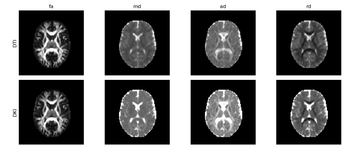
The fit method creates a DiffusionKurtosisFit object, which contains all the diffusion and kurtosis fitting parameters and other DKI attributes. For instance, since the diffusion kurtosis model estimates the diffusion tensor, all standard diffusion tensor statistics can be computed from the DiffusionKurtosisFit instance. For example, we can extract the fractional anisotropy (FA), the mean diffusivity (MD), the radial diffusivity (RD) and the axial diffusivity (AD) from the DiffusionKurtosisiFit instance. Of course, these measures can also be computed from DIPY’s TensorModel fit, and should be analogous; however, theoretically, the diffusion statistics from the kurtosis model are expected to have better accuracy, since DKI’s diffusion tensor are decoupled from higher order terms effects [8], [2]. Below we compare the FA, MD, AD, and RD, computed from both DTI and DKI.

tenmodel = dti.TensorModel(gtab)
tenfit = tenmodel.fit(data[:, :, 9:10], mask=mask[:, :, 9:10])

fits = [tenfit, dkifit]
maps = ["fa", "md", "rd", "ad"]
fit_labels = ["DTI", "DKI"]
map_kwargs = [{"vmax": 0.7}, {"vmax": 2e-3}, {"vmax": 2e-3}, {"vmax": 2e-3}]
compare_maps(
    fits,
    maps,
    fit_labels=fit_labels,
    map_kwargs=map_kwargs,
    filename="Diffusion_tensor_measures_from_DTI_and_DKI.png",
)

Diffusion tensor measures obtained from the diffusion tensor estimated from DKI (upper panels) and DTI (lower panels).

DTI’s diffusion estimates present lower values than DKI’s estimates, showing that DTI’s diffusion measurements are underestimated by higher order effects (for detailed discussion on this see [2].

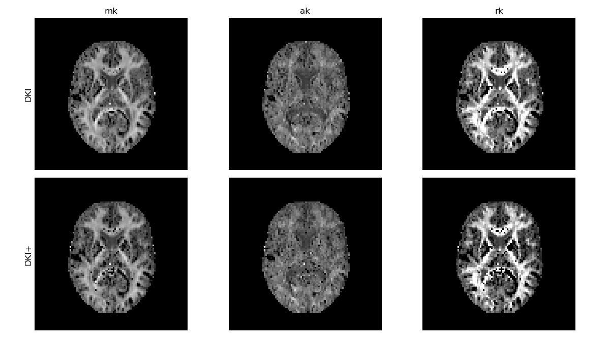
In addition to the standard diffusion statistics, the DiffusionKurtosisFit instance can be used to estimate the non-Gaussian measures of mean kurtosis (MK), the radial kurtosis (RK) and the axial kurtosis (AK).

maps = ["mk", "rk", "ak"]
compare_maps(
    [dkifit],
    maps,
    fit_labels=["DKI"],
    map_kwargs={"vmin": 0, "vmax": 1.5},
    filename="DKI_standard_measures.png",
)

DKI standard kurtosis measures.

The non-Gaussian behaviour of the diffusion signal is expected to be higher when tissue water is confined by multiple compartments. MK is, therefore, higher in white matter since it is highly compartmentalized by myelin sheaths. These water diffusion compartmentalization is expected to be more pronounced perpendicularly to white matter fibers and thus the RK map presents higher amplitudes than the AK map.

Mitigating ‘Black’ Voxels / Holes in DKI metrics

It is important to note that kurtosis estimates might present implausible negative estimates in deep white matter regions that will manifest as ‘Black’ voxels or holes in DKI metrics (e.g. see the band of dark voxels in the RK map above). These negative kurtosis values are artifactual and might be induced by: 1) low radial diffusivities of aligned white matter - since it is very hard to capture non-Gaussian information in radial direction due to its low diffusion decays, radial kurtosis estimates (and consequently the mean kurtosis estimates) might have low robustness and tendency to exhibit negative values [6], [7]; 2) Gibbs artifacts - MRI images might be corrupted by signal oscillation artifact between tissue’s edges if an inadequate number of high frequencies of the k-space is sampled. These oscillations might have different signs on images acquired with different diffusion-weighted and inducing negative biases in kurtosis parametric maps [9], [10]. 3) Underestimation of b0 signals - Due to physiological or noise artifacts, the signals acquired at b-value=0 may be artifactually lower than the diffusion-weighted signals acquired for the different b-values. In this case, the log diffusion-weighted signal decay may appear to be concave rather than showing to be convex (as one would typically expect), leading to negative kurtosis value estimates.

Given the above, one can try to suppress the ‘Black’ voxel / holes in DKI metrics by: 1) using more advanced noise and artifact suppression algorithms, e.g., as mentioned above, the MP-PCA denoising (Denoise images using the Marcenko-Pastur PCA algorithm), other denoising alternatives such as Patch2self (Patch2Self: Self-Supervised Denoising via Statistical Independence) or incorporating methods for Gibbs Artifact Unringing (Suppress Gibbs oscillations) algorithms. 2) computing the kurtosis values from powder-averaged diffusion-weighted signals which are known to be less sensitive to implausible negative estimates. The details on how to compute the kurtosis from powder-averaged signals in DIPY are described in the following tutorial (Mean signal diffusion kurtosis imaging (MSDKI)). 3) computing alternative definitions of mean and radial kurtosis such as the mean kurtosis tensor (MKT) and radial tensor kurtosis (RTK) metrics (see below). 4) constrained optimization to ensure that the fitted parameters are physically plausible [11] (see below).

Alternative DKI metrics

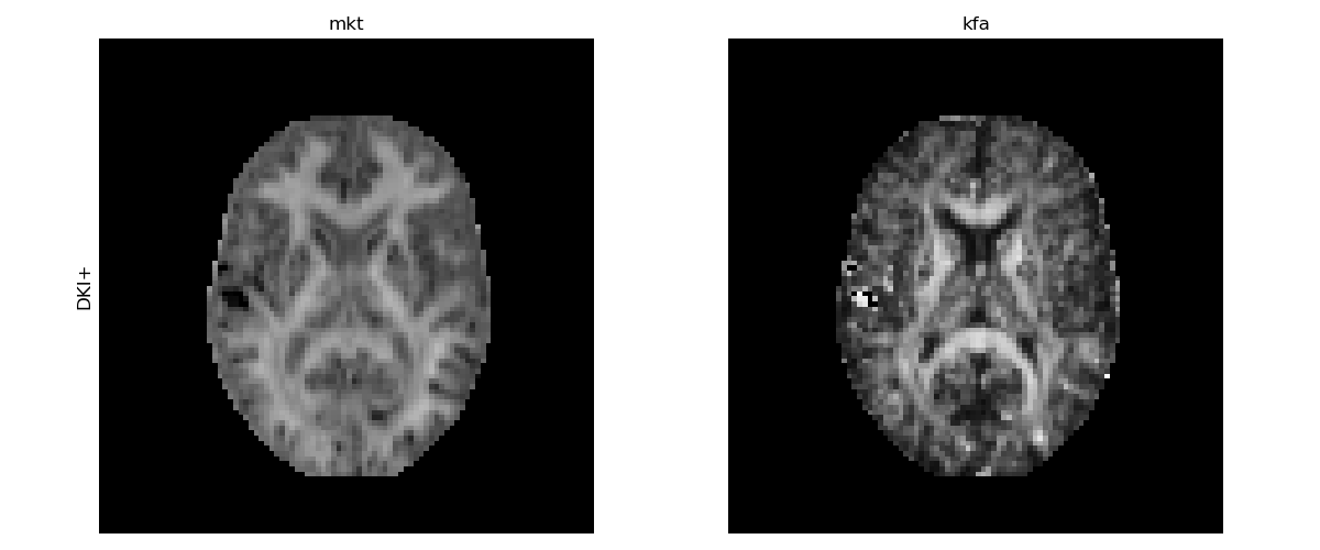
In addition to the standard mean, axial, and radial kurtosis metrics shown above, alternative metrics can be computed from DKI, e.g.: 1) the mean kurtosis tensor (MKT) - defined as the trace of the kurtosis tensor - is a quantity that provides a contrast similar to the standard MK but it is more robust to noise artifacts [12], [2]. 2) the radial tensor kurtosis (RTK) provides an alternative definition to standard radial kurtosis (RK) that, as MKT, is more robust to noise artifacts [12]. 3) the kurtosis fractional anisotropy (KFA) that quantifies the anisotropy of the kurtosis tensor [13], which provides different information than the FA measures from the diffusion tensor.

These measures are computed and illustrated below:

compare_maps(
    [dkifit],
    ["mkt", "rtk", "kfa"],
    fit_labels=["DKI"],
    map_kwargs=[
        {"vmin": 0, "vmax": 1.5},
        {"vmin": 0, "vmax": 1.5},
        {"vmin": 0, "vmax": 1},
    ],
    filename="Alternative_DKI_metrics.png",
)

Alternative DKI measures.

Constrained optimization for DKI

When instantiating the DiffusionKurtosisModel, the model can be set up to use constraints with the option fit_method=’CLS’ (for ordinary least squares) or with fit_method=’CWLS’ (for weighted least squares). Constrained fitting takes more time than unconstrained fitting, but is generally recommended to prevent physically implausible parameter estimates [11]. For performance purposes it is recommended to use the MOSEK solver (https://www.mosek.com/) by setting cvxpy_solver='MOSEK'. Different solvers can differ greatly in terms of runtime and solution accuracy, and in some cases solvers may show warnings about convergence or recommended option settings.

Note

In certain atypical scenarios, the DKI+ constraints could potentially be too restrictive. Always check the results of a constrained fit with their unconstrained counterpart to verify that there are no unexpected qualitative differences.

dkimodel_plus = dki.DiffusionKurtosisModel(gtab, fit_method="CLS")
dkifit_plus = dkimodel_plus.fit(data[:, :, 9:10], mask=mask[:, :, 9:10])

/opt/homebrew/Caskroom/miniforge/base/envs/py312-test/lib/python3.12/site-packages/cvxpy/problems/problem.py:1481: UserWarning: Solution may be inaccurate. Try another solver, adjusting the solver settings, or solve with verbose=True for more information.
  warnings.warn(
/opt/homebrew/Caskroom/miniforge/base/envs/py312-test/lib/python3.12/site-packages/dipy/testing/decorators.py:192: UserWarning: Solver failed to produce an optimum: optimal_inaccurate.
  return func(*args, **kwargs)

We can now compare the kurtosis measures obtained with the constrained fit to the measures obtained before, where we see that many of the artifactual voxels have now been corrected. In particular outliers caused by pure noise – instead of for example acquisition artifacts – can be corrected with this method.

compare_maps(
    [dkifit, dkifit_plus],
    ["mkt", "rtk", "ak"],
    fit_labels=["DKI", "DKI+"],
    map_kwargs={"vmin": 0, "vmax": 1.5},
    filename="Alternative_DKI_measures_comparison_to_DKIplus.png",
)

DKI standard kurtosis measures obtained with constrained optimization.

References

[1]

Jens H. Jensen, Joseph A. Helpern, Anita Ramani, Hanzhang Lu, and Kyle Kaczynski. Diffusional kurtosis imaging: The quantification of non-gaussian water diffusion by means of magnetic resonance imaging. Magnetic Resonance in Medicine, 53(6):1432–1440, 2005. URL: https://onlinelibrary.wiley.com/doi/abs/10.1002/mrm.20508, doi:https://doi.org/10.1002/mrm.20508.

[2] (1,2,3,4,5,6)

Rafael Neto Henriques, Marta M. Correia, Maurizio Marrale, Elizabeth Huber, John Kruper, Serge Koudoro, Jason D. Yeatman, Eleftherios Garyfallidis, and Ariel Rokem. Diffusional Kurtosis Imaging in the Diffusion Imaging in Python Project. Frontiers in Human Neuroscience, July 2021. Sec. Brain Imaging and Stimulation. Advanced Diffusion MRI for Brain Microstructure: Methodology, Consistency, and Application. URL: https://doi.org/10.3389/fnhum.2021.675433, doi:10.3389/fnhum.2021.675433.

[3]

Rafael Neto Henriques, Marta Morgado Correia, Rita Gouveia Nunes, and Hugo Alexandre Ferreira. Exploring the 3D geometry of the diffusion kurtosis tensor—Impact on the development of robust tractography procedures and novel biomarkers. NeuroImage, 111:85–99, 2015. URL: https://doi.org/10.1016/j.neuroimage.2015.02.004, doi:10.1016/j.neuroimage.2015.02.004.

[4]

Brian Hansen and Sune Nørhøj Jespersen. Data for evaluation of fast kurtosis strategies, b-value optimization and exploration of diffusion MRI contrast. Scientific Data, 3(1):160072, August 2016. URL: https://doi.org/10.1038/sdata.2016.72, doi:10.1038/sdata.2016.72.

[5]

Chantal M.W. Tax, Willem M. Otte, Max A. Viergever, Rick M. Dijkhuizen, and Alexander Leemans. REKINDLE: Robust extraction of kurtosis INDices with linear estimation. Magnetic Resonance in Medicine, 73(2):794–808, 2015. URL: https://doi.org/10.1002/mrm.25165, doi:10.1002/mrm.25165.

[6] (1,2)

Rafael Neto Henriques. Diffusion kurtosis imaging of the healthy human brain. Master’s thesis, Universidade de Lisboa, Lisboa, Portugal, 2012. URL: https://repositorio.ul.pt/bitstream/10451/8511/1/ulfc104137_tm_Rafael_Henriques.pdf, doi:.

[7] (1,2)

Ali Tabesh, Jens H. Jensen, Babak A. Ardekani, and Joseph A. Helpern. Estimation of tensors and tensor-derived measures in diffusional kurtosis imaging. Magnetic Resonance in Medicine, 65(3):823–836, 2011. URL: https://doi.org/10.1002/mrm.22655, doi:10.1002/mrm.22655.

[8]

Jelle Veraart, Dirk H. J. Poot, Wim Van Hecke, Ines Blockx, Annemie Van der Linden, Marleen Verhoye, and Jan Sijbers. More accurate estimation of diffusion tensor parameters using diffusion kurtosis imaging. Magnetic Resonance in Medicine, 65(1):138–145, 2011. URL: https://doi.org/10.1002/mrm.22603, doi:10.1002/mrm.22603.

[9]

Daniele Perrone, Jan Aelterman, Aleksandra Pižurica, Ben Jeurissen, Wilfried Philips, and Alexander Leemans. The effect of Gibbs ringing artifacts on measures derived from diffusion MRI. NeuroImage, 120:441–455, 2015. URL: https://doi.org/10.1016/j.neuroimage.2015.06.068, doi:10.1016/j.neuroimage.2015.06.068.

[10]

Rafael Neto Henriques. Advanced Methods for Diffusion MRI Data Analysis and their Application to the Healthy Ageing Brain. PhD thesis, Cambridge University, Cambridge, United Kingdom, 2018. URL: https://doi.org/10.17863/CAM.29356, doi:10.17863/CAM.29356.

[11] (1,2)

Tom Dela Haije, Evren Özarslan, and Aasa Feragen. Enforcing necessary non-negativity constraints for common diffusion MRI models using sum of squares programming. NeuroImage, 209:116405, 2020. URL: https://doi.org/10.1016/j.neuroimage.2019.116405, doi:10.1016/j.neuroimage.2019.116405.

[12] (1,2)

Brian Hansen, Torben E. Lund, Ryan Sangill, and Sune Nørhøj Jespersen. Experimentally and computationally fast method for estimation of a mean kurtosis. Magnetic Resonance in Medicine, 69(6):1754–1760, 2013. URL: https://doi.org/10.1002/mrm.24743, doi:10.1002/mrm.24743.

[13]

G. Russell Glenn, Joseph A. Helpern, Ali Tabesh, and Jens H. Jensen. Quantitative assessment of diffusional kurtosis anisotropy. NMR in Biomedicine, 28(4):448–459, 2015. URL: https://doi.org/10.1002/nbm.3271, doi:10.1002/nbm.3271.