Local reconstruction using the Histological ResDNN

A data-driven approach to modeling the non-linear mapping between observed DW-MRI signals and ground truth structures using sequential deep neural network regression with residual block deep neural network (ResDNN) [1], [2].

Training was performed on two 3-D histology datasets of squirrel monkey brains and validated on a third. A second validation was performed on HCP datasets.

import os

import numpy as np
import scipy.ndimage as ndi

from dipy.core.gradients import gradient_table
from dipy.data import get_fnames, get_sphere
from dipy.io.gradients import read_bvals_bvecs
from dipy.io.image import load_nifti, save_nifti
from dipy.nn.histo_resdnn import HistoResDNN
from dipy.reconst.shm import sh_to_sf_matrix
from dipy.segment.mask import median_otsu
from dipy.viz import actor, window

# Disable oneDNN warning
os.environ["TF_CPP_MIN_LOG_LEVEL"] = "2"

This ResDNN model requires single-shell data with one or more b0s, the data is fetched and a gradient table is constructed from bvals/bvecs.

# Fetch DWI and GTAB
hardi_fname, hardi_bval_fname, hardi_bvec_fname = get_fnames(name="stanford_hardi")
data, affine = load_nifti(hardi_fname)
data = np.squeeze(data)
bvals, bvecs = read_bvals_bvecs(hardi_bval_fname, hardi_bvec_fname)
gtab = gradient_table(bvals, bvecs=bvecs)

To accelerate computation, a brain mask must be computed. The resulting mask is saved for visual inspection.

mean_b0 = data[..., gtab.b0s_mask]
mean_b0 = np.mean(mean_b0, axis=-1)
_, mask = median_otsu(mean_b0)

mask_labeled, _ = ndi.label(mask)
unique, count = np.unique(mask_labeled, return_counts=True)
val = unique[np.argmax(count[1:]) + 1]
mask[mask_labeled != val] = 0

save_nifti("mask.nii.gz", mask.astype(np.uint8), affine)

Using a ResDNN for sh_order_max 8 (default) and load the appropriate weights. Fit the data and save the resulting fODF.

resdnn_model = HistoResDNN(verbose=True)
resdnn_model.fetch_default_weights()
predicted_sh = resdnn_model.predict(data, gtab, mask=mask)

save_nifti("predicted_sh.nii.gz", predicted_sh, affine)

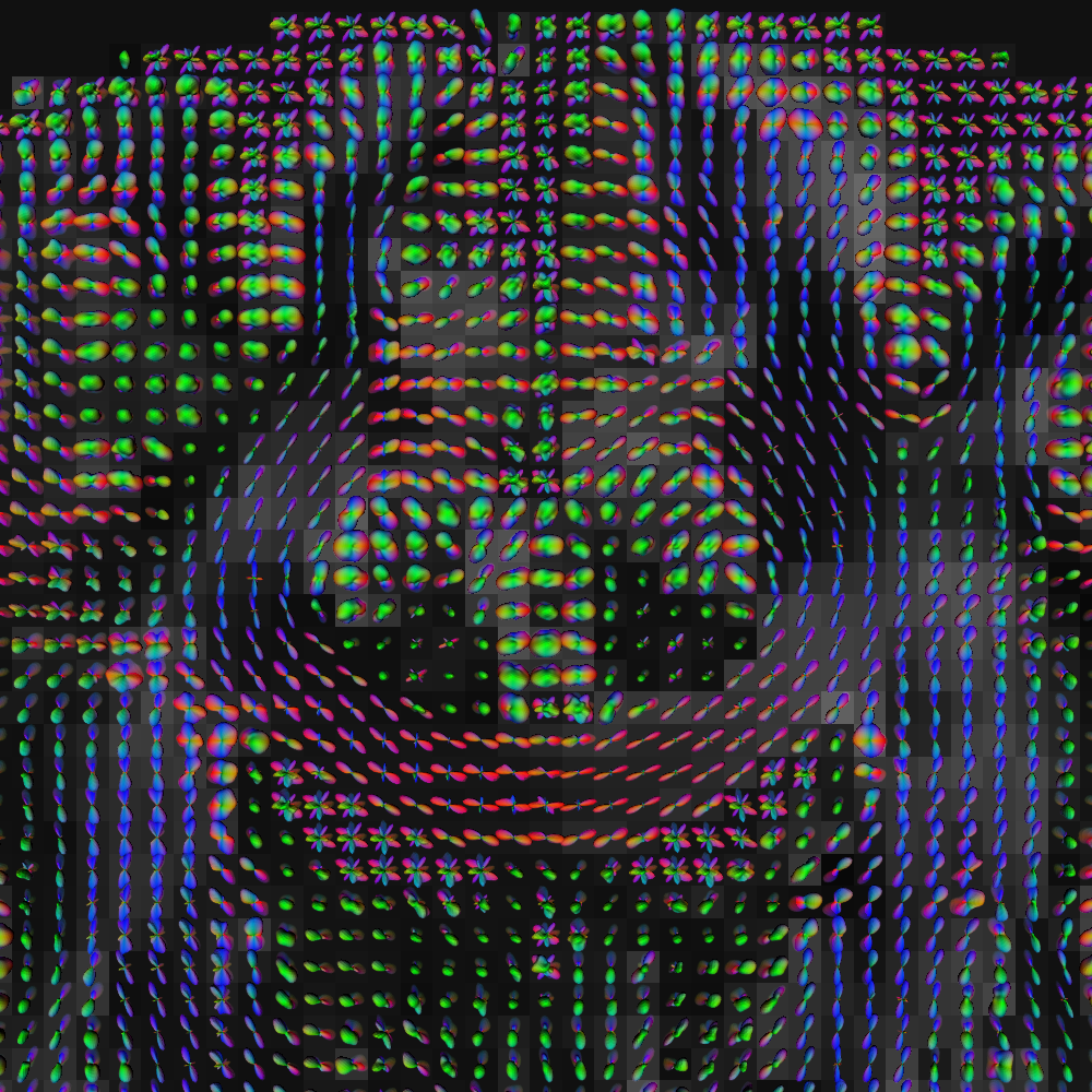
Preparing the scene using FURY. The ODF slicer and the background image are added as actors and a mid-coronal slice is selected.

interactive = False
sphere = get_sphere(name="repulsion724")
B, invB = sh_to_sf_matrix(
    sphere, sh_order_max=8, basis_type=resdnn_model.basis_type, smooth=0.0006
)
fod_spheres = actor.odf_slicer(
    predicted_sh, sphere=sphere, scale=0.6, norm=True, mask=mask, B_matrix=B
)

mean_sh = np.mean(predicted_sh, axis=-1)
background_img = actor.slicer(mean_sh, opacity=0.5, interpolation="nearest")

# Select the mid coronal slice for slicer
ori_shape = mask.shape[0:3]
slice_index = ori_shape[1] // 2
fod_spheres.display_extent(0, ori_shape[0], slice_index, slice_index, 0, ori_shape[2])
background_img.display_extent(
    0, ori_shape[0], slice_index, slice_index, 0, ori_shape[2]
)

scene = window.Scene()
scene.add(fod_spheres)
scene.add(background_img)

Adjusting the camera for a nice zoom-in of the corpus callosum (coronal) to screenshot the resulting prediction. FODF should be aligned with the curvature of the corpus callosum and a single-fiber population should be visible.

camera = {
    "zoom_factor": 0.85,
    "view_position": np.array(
        [(ori_shape[0] - 1) / 2.0, max(ori_shape), (ori_shape[2] - 1) / 1.5]
    ),
    "view_center": np.array(
        [(ori_shape[0] - 1) / 2.0, slice_index, (ori_shape[2] - 1) / 1.5]
    ),
    "up_vector": np.array([0.0, 0.0, 1.0]),
}

scene.set_camera(
    position=camera["view_position"],
    focal_point=camera["view_center"],
    view_up=camera["up_vector"],
)
scene.zoom(camera["zoom_factor"])

if interactive:
    window.show(scene, reset_camera=False)

window.record(
    scene=scene, out_path="pred_fODF.png", size=(1000, 1000), reset_camera=False
)

Visualization of the predicted fODF.

References

[1]

Vishwesh Nath, Kurt G. Schilling, Prasanna Parvathaneni, Allison E. Hainline, Colin B. Hansen, Camilo Bermudez, Andrew J. Plassard, Justin A. Blaber, Vaibhav Janve, Yurui Gao, Iwona Stepniewska, Adam W. Anderson, and Bennett A. Landman. Deep Learning Captures More Accurate Diffusion Fiber Orientations Distributions than Constrained Spherical Deconvolution. In Joint Annual Meeting ISMRM-ESMRMB 2018 SMRT 27th Annual Meeting. Paris, France, 2018. International Society for Magnetic Resonance in Medicine (ISMRM).

[2]

Vishwesh Nath, Kurt G. Schilling, Prasanna Parvathaneni, Colin B. Hansen, Allison E. Hainline, Yuankai Huo, Justin A. Blaber, Ilwoo Lyu, Vaibhav Janve, Yurui Gao, Iwona Stepniewska, Adam W. Anderson, and Bennett A. Landman. Deep learning reveals untapped information for local white-matter fiber reconstruction in diffusion-weighted MRI. Magnetic Resonance Imaging, 62:220–227, 2019. URL: https://doi.org/10.1016/j.mri.2019.07.012, doi:10.1016/j.mri.2019.07.012.