Reconstruct with Constant Solid Angle (Q-Ball)

We show how to apply a Constant Solid Angle ODF (Q-Ball) model from Aganj et al. [Aganj2010] to your datasets.

First import the necessary modules:

import numpy as np

from dipy.core.gradients import gradient_table
from dipy.data import get_fnames, default_sphere
from dipy.io.gradients import read_bvals_bvecs
from dipy.io.image import load_nifti
from dipy.reconst.shm import CsaOdfModel
from dipy.direction import peaks_from_model
from dipy.segment.mask import median_otsu
from dipy.viz import window, actor

Download and read the data for this tutorial and load the raw diffusion data and the affine.

hardi_fname, hardi_bval_fname, hardi_bvec_fname = get_fnames('stanford_hardi')

data, affine = load_nifti(hardi_fname)

bvals, bvecs = read_bvals_bvecs(hardi_bval_fname, hardi_bvec_fname)
gtab = gradient_table(bvals, bvecs)

img contains a nibabel Nifti1Image object (data) and gtab contains a GradientTable object (gradient information e.g. b-values). For example to read the b-values it is possible to write print(gtab.bvals).

print('data.shape (%d, %d, %d, %d)' % data.shape)

data.shape (81, 106, 76, 160)

Remove most of the background using DIPY’s mask module.

maskdata, mask = median_otsu(data, vol_idx=range(10, 50), median_radius=3,
                             numpass=1, autocrop=True, dilate=2)

We instantiate our CSA model with spherical harmonic order (l) of 4

csamodel = CsaOdfModel(gtab, 4)

Peaks_from_model is used to calculate properties of the ODFs (Orientation Distribution Function) and return for example the peaks and their indices, or GFA which is similar to FA but for ODF based models. This function mainly needs a reconstruction model, the data and a sphere as input. The sphere is an object that represents the spherical discrete grid where the ODF values will be evaluated.

csapeaks = peaks_from_model(model=csamodel,
                            data=maskdata,
                            sphere=default_sphere,
                            relative_peak_threshold=.5,
                            min_separation_angle=25,
                            mask=mask,
                            return_odf=False,
                            normalize_peaks=True)

GFA = csapeaks.gfa

print('GFA.shape (%d, %d, %d)' % GFA.shape)

GFA.shape (71, 88, 62)

Apart from GFA, csapeaks also has the attributes peak_values, peak_indices and ODF. peak_values shows the maxima values of the ODF and peak_indices gives us their position on the discrete sphere that was used to do the reconstruction of the ODF. In order to obtain the full ODF, return_odf should be True. Before enabling this option, make sure that you have enough memory.

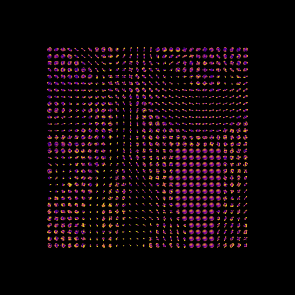
Let’s visualize the ODFs of a small rectangular area in an axial slice of the splenium of the corpus callosum (CC).

data_small = maskdata[13:43, 44:74, 28:29]

# Enables/disables interactive visualization
interactive = False

scene = window.Scene()

csaodfs = csamodel.fit(data_small).odf(default_sphere)

It is common with CSA ODFs to produce negative values, we can remove those using np.clip

csaodfs = np.clip(csaodfs, 0, np.max(csaodfs, -1)[..., None])
csa_odfs_actor = actor.odf_slicer(csaodfs, sphere=default_sphere,
                                  colormap='plasma', scale=0.4)
csa_odfs_actor.display(z=0)

scene.add(csa_odfs_actor)
print('Saving illustration as csa_odfs.png')
window.record(scene, n_frames=1, out_path='csa_odfs.png', size=(600, 600))
if interactive:
    window.show(scene)

Saving illustration as csa_odfs.png

Constant Solid Angle ODFs.

References

[Aganj2010]

Aganj I, Lenglet C, Sapiro G, Yacoub E, Ugurbil K, Harel N. “Reconstruction of the orientation distribution function in single- and multiple-shell q-ball imaging within constant solid angle”, Magnetic Resonance in Medicine. 2010 Aug;64(2):554-66. doi: 10.1002/mrm.22365