Visualization of ROI Surface Rendered with Streamlines

Here is a simple tutorial following the probabilistic CSA Tracking Example in which we generate a dataset of streamlines from a corpus callosum ROI, and then display them with the seed ROI rendered in 3D with 50% transparency.

Let’s start by importing the relevant modules.

from dipy.core.gradients import gradient_table
from dipy.reconst.shm import CsaOdfModel
from dipy.data import default_sphere, get_fnames
from dipy.direction import peaks_from_model
from dipy.io.gradients import read_bvals_bvecs
from dipy.io.image import load_nifti, load_nifti_data
from dipy.tracking.stopping_criterion import ThresholdStoppingCriterion
from dipy.tracking import utils
from dipy.tracking.local_tracking import LocalTracking
from dipy.tracking.streamline import Streamlines
from dipy.viz import actor, window, colormap as cmap

First, we need to generate some streamlines. For a more complete description of these steps, please refer to the CSA Probabilistic Tracking Tutorial.

hardi_fname, hardi_bval_fname, hardi_bvec_fname = get_fnames('stanford_hardi')
label_fname = get_fnames('stanford_labels')

data, affine, hardi_img = load_nifti(hardi_fname, return_img=True)
labels = load_nifti_data(label_fname)
bvals, bvecs = read_bvals_bvecs(hardi_bval_fname, hardi_bvec_fname)
gtab = gradient_table(bvals, bvecs)

white_matter = (labels == 1) | (labels == 2)

csa_model = CsaOdfModel(gtab, sh_order_max=6)
csa_peaks = peaks_from_model(csa_model, data, default_sphere,
                             relative_peak_threshold=.8,
                             min_separation_angle=45,
                             mask=white_matter)

stopping_criterion = ThresholdStoppingCriterion(csa_peaks.gfa, .25)

seed_mask = labels == 2
seeds = utils.seeds_from_mask(seed_mask, affine, density=[1, 1, 1])

# Initialization of LocalTracking. The computation happens in the next step.
streamlines = LocalTracking(csa_peaks, stopping_criterion, seeds, affine,
                            step_size=2)

# Compute streamlines and store as a list.
streamlines = Streamlines(streamlines)

We will create a streamline actor from the streamlines.

streamlines_actor = actor.line(streamlines, cmap.line_colors(streamlines))

Next, we create a surface actor from the corpus callosum seed ROI. We provide the ROI data, the affine, the color in [R,G,B], and the opacity as a decimal between zero and one. Here, we set the color as blue/green with 50% opacity.

surface_opacity = 0.5
surface_color = [0, 1, 1]

seedroi_actor = actor.contour_from_roi(seed_mask, affine,
                                       surface_color, surface_opacity)

Next, we initialize a ‘’Scene’’ object and add both actors to the rendering.

scene = window.Scene()
scene.add(streamlines_actor)
scene.add(seedroi_actor)

If you uncomment the following line, the rendering will pop up in an interactive window.

interactive = False
if interactive:
    window.show(scene)

window.record(scene, out_path='contour_from_roi_tutorial.png', size=(1200, 900))

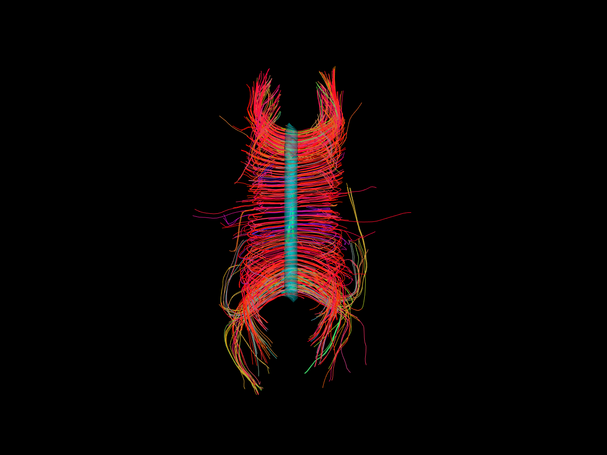
A top view of corpus callosum streamlines with the blue transparent seed ROI in the center.