Using the RESTORE algorithm for robust tensor fitting

The diffusion tensor model takes into account certain kinds of noise (thermal), but not other kinds, such as “physiological” noise. For example, if a subject moves during acquisition of one of the diffusion-weighted samples, this might have a substantial effect on the parameters of the tensor fit calculated in all voxels in the brain for that subject. One of the pernicious consequences of this is that it can lead to wrong interpretation of group differences. For example, some groups of participants (e.g. young children, patient groups, etc.) are particularly prone to motion and differences in tensor parameters and derived statistics (such as FA) due to motion would be confounded with actual differences in the physical properties of the white matter. An example of this was shown in a paper by Yendiki et al. [Yendiki2013].

One of the strategies to deal with this problem is to apply an automatic method for detecting outliers in the data, excluding these outliers and refitting the model without the presence of these outliers. This is often referred to as “robust model fitting”. One of the common algorithms for robust tensor fitting is called RESTORE, and was first proposed by Chang et al. [Chang2005].

In the following example, we will demonstrate how to use RESTORE on a simulated dataset, which we will corrupt by adding intermittent noise.

We start by importing a few of the libraries we will use.

• The module dipy.reconst.dti contains the implementation of tensor fitting, including an implementation of the RESTORE algorithm.

• The module dipy.data is used for small datasets that we use in tests and examples.

• dipy.io.image is for loading / saving imaging datasets

• dipy.io.gradients is for loading / saving our bvals and bvecs

• dipy.viz package is used for 3D visualization and matplotlib for 2D visualizations:

import numpy as np
import matplotlib.pyplot as plt

from dipy.core.gradients import gradient_table
import dipy.data as dpd
import dipy.denoise.noise_estimate as ne
from dipy.io.image import load_nifti
from dipy.io.gradients import read_bvals_bvecs
import dipy.reconst.dti as dti
from dipy.viz import window, actor

# Enables/disables interactive visualization
interactive = False

If needed, the fetch_stanford_hardi function will download the raw dMRI dataset of a single subject. The size of this dataset is 87 MBytes. You only need to fetch once.

hardi_fname, hardi_bval_fname, hardi_bvec_fname = dpd.get_fnames(
    'stanford_hardi')
data, affine = load_nifti(hardi_fname)

bvals, bvecs = read_bvals_bvecs(hardi_bval_fname, hardi_bvec_fname)
gtab = gradient_table(bvals, bvecs)

We initialize a DTI model class instance using the gradient table used in the measurement. By default, dti.TensorModel will use a weighted least-squares algorithm (described in [Chang2005]) to fit the parameters of the model. We initialize this model as a baseline for comparison of noise-corrupted models:

dti_wls = dti.TensorModel(gtab)

For the purpose of this example, we will focus on the data from a region of interest (ROI) surrounding the Corpus Callosum. We define that ROI as the following indices:

roi_idx = (slice(20, 50), slice(55, 85), slice(38, 39))

And use them to index into the data:

data = data[roi_idx]

This dataset is not very noisy, so we will artificially corrupt it to simulate the effects of “physiological” noise, such as subject motion. But first, let’s establish a baseline, using the data as it is:

fit_wls = dti_wls.fit(data)

fa1 = fit_wls.fa
evals1 = fit_wls.evals
evecs1 = fit_wls.evecs
cfa1 = dti.color_fa(fa1, evecs1)
sphere = dpd.default_sphere

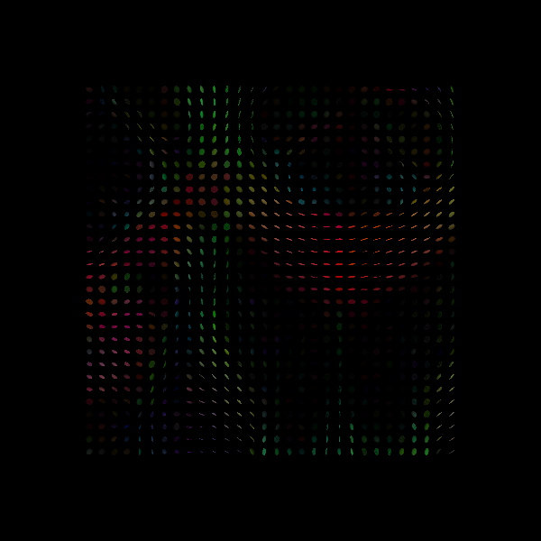
We visualize the ODFs in the ROI using dipy.viz module:

scene = window.Scene()
scene.add(actor.tensor_slicer(evals1, evecs1, scalar_colors=cfa1,
                              sphere=sphere, scale=0.3))
window.record(scene, out_path='tensor_ellipsoids_wls.png', size=(600, 600))
if interactive:
    window.show(scene)

Tensor Ellipsoids.

scene.clear()

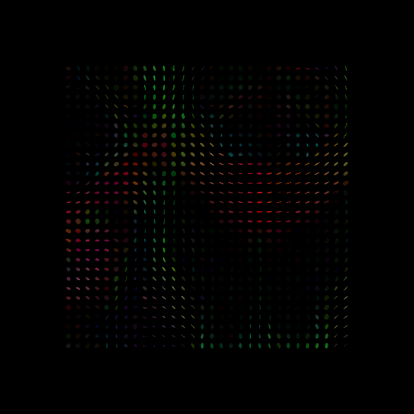
Next, we corrupt the data with some noise. To simulate a subject that moves intermittently, we will replace a few of the images with a very low signal

noisy_data = np.copy(data)
noisy_idx = slice(-10, None)  # The last 10 volumes are corrupted
noisy_data[..., noisy_idx] = 1.0

We use the same model to fit this noisy data

fit_wls_noisy = dti_wls.fit(noisy_data)
fa2 = fit_wls_noisy.fa
evals2 = fit_wls_noisy.evals
evecs2 = fit_wls_noisy.evecs
cfa2 = dti.color_fa(fa2, evecs2)

scene = window.Scene()
scene.add(actor.tensor_slicer(evals2, evecs2, scalar_colors=cfa2,
                              sphere=sphere, scale=0.3))
window.record(scene, out_path='tensor_ellipsoids_wls_noisy.png',
              size=(600, 600))
if interactive:
    window.show(scene)

In places where the tensor model is particularly sensitive to noise, the resulting tensor field will be distorted

Tensor Ellipsoids from noisy data.

To estimate the parameters from the noisy data using RESTORE, we need to estimate what would be a reasonable amount of noise to expect in the measurement. To do that, we use the dipy.denoise.noise_estimate module:

sigma = ne.estimate_sigma(data)

This estimate of the standard deviation will be used by the RESTORE algorithm to identify the outliers in each voxel and is given as an input when initializing the TensorModel object:

dti_restore = dti.TensorModel(gtab, fit_method='RESTORE', sigma=sigma)
fit_restore_noisy = dti_restore.fit(noisy_data)
fa3 = fit_restore_noisy.fa
evals3 = fit_restore_noisy.evals
evecs3 = fit_restore_noisy.evecs
cfa3 = dti.color_fa(fa3, evecs3)

scene = window.Scene()
scene.add(actor.tensor_slicer(evals3, evecs3, scalar_colors=cfa3,
                              sphere=sphere, scale=0.3))
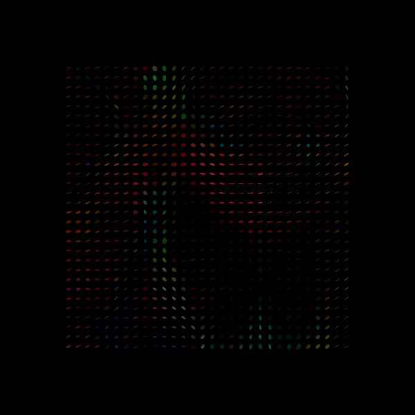
print('Saving illustration as tensor_ellipsoids_restore_noisy.png')
window.record(scene, out_path='tensor_ellipsoids_restore_noisy.png',
              size=(600, 600))
if interactive:
    window.show(scene)

Saving illustration as tensor_ellipsoids_restore_noisy.png

# Tensor Ellipsoids from noisy data recovered with RESTORE.


# The tensor field looks rather restored to its noiseless state in this
# image, but to convince ourselves further that this did the right thing, we
# will compare  the distribution of FA in this region relative to the
# baseline, using the RESTORE estimate and the WLS estimate [Chung2006]_.

fig_hist, ax = plt.subplots(1)
ax.hist(np.ravel(fa2), color='b', histtype='step', label='WLS')
ax.hist(np.ravel(fa3), color='r', histtype='step', label='RESTORE')
ax.hist(np.ravel(fa1), color='g', histtype='step', label='Original')
ax.set_xlabel('Fractional Anisotropy')
ax.set_ylabel('Count')
plt.legend()
fig_hist.savefig('dti_fa_distributions.png')

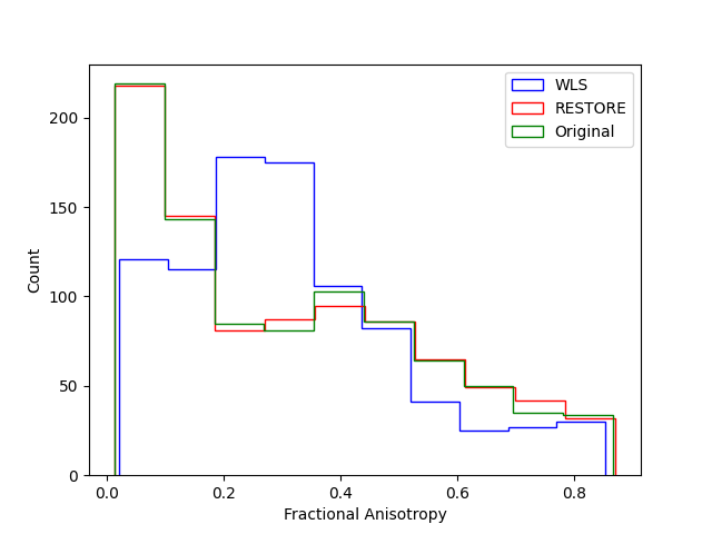
This demonstrates that RESTORE can recover a distribution of FA that more closely resembles the baseline distribution of the noiseless signal, and demonstrates the utility of the method to data with intermittent noise. Importantly, this method assumes that the tensor is a good representation of the diffusion signal in the data. If you have reason to believe this is not the case (for example, you have data with very high b values and you are particularly interested in locations in the brain in which fibers cross), you might want to use a different method to fit your data.

References

[Yendiki2013]

Yendiki, A, Koldewynb, K, Kakunooria, S, Kanwisher, N, and Fischl, B. (2013). Spurious group differences due to head motion in a diffusion MRI study. Neuroimage.

[Chang2005] (1,2)

Chang, L-C, Jones, DK and Pierpaoli, C (2005). RESTORE: robust estimation of tensors by outlier rejection. MRM, 53: 1088-95.

[Chung2006]

Chung, SW, Lu, Y, Henry, R-G, (2006). Comparison of bootstrap approaches for estimation of uncertainties of DTI parameters. NeuroImage 33, 531-541.