K-fold cross-validation for model comparison

Different models of diffusion MRI can be compared based on their accuracy in fitting the diffusion signal. Here, we demonstrate this by comparing two models: the diffusion tensor model (DTI) and Constrained Spherical Deconvolution (CSD). These models differ from each other substantially. DTI approximates the diffusion pattern as a 3D Gaussian distribution, and has only 6 free parameters. CSD, on the other hand, fits many more parameters. The models are also not nested, so they cannot be compared using the log-likelihood ratio.

A general way to perform model comparison is cross-validation [1]. In this method, a model is fit to some of the data (a learning set) and the model is then used to predict a held-out set (a testing set). The model predictions can then be compared to estimate prediction error on the held out set. This method has been used for comparison of models such as DTI and CSD [2], and has the advantage that it the comparison is imprevious to differences in the number of in the model, and it can be used to compare models that are not nested.

In DIPY, we include an implementation of k-fold cross-validation. In this method, the data is divided into \(k\) different segments. In each iteration :math:` rac{1}{k}th` of the data is held out and the model is fit to the other :math:` rac{k-1}{k}` parts of the data. A prediction of the held out data is done and recorded. At the end of \(k\) iterations a prediction of all of the data will have been conducted, and this can be compared directly to all of the data.

First, we import that modules needed for this example. In particular, the reconst.cross_validation module implements k-fold cross-validation

import matplotlib.pyplot as plt
import numpy as np
import scipy.stats as stats

from dipy.core.gradients import gradient_table
import dipy.data as dpd
from dipy.io.gradients import read_bvals_bvecs
from dipy.io.image import load_nifti
import dipy.reconst.cross_validation as xval
import dipy.reconst.csdeconv as csd
import dipy.reconst.dti as dti

np.random.seed(2014)

We fetch some data and select a couple of voxels to perform comparisons on. One lies in the corpus callosum (cc), while the other is in the centrum semiovale (cso), a part of the brain known to contain multiple crossing white matter fiber populations.

hardi_fname, hardi_bval_fname, hardi_bvec_fname = dpd.get_fnames(name="stanford_hardi")

data, affine = load_nifti(hardi_fname)
bvals, bvecs = read_bvals_bvecs(hardi_bval_fname, hardi_bvec_fname)
gtab = gradient_table(bvals, bvecs=bvecs)


cc_vox = data[40, 70, 38]
cso_vox = data[30, 76, 38]

We initialize each kind of model:

dti_model = dti.TensorModel(gtab)
response, ratio = csd.auto_response_ssst(gtab, data, roi_radii=10, fa_thr=0.7)
csd_model = csd.ConstrainedSphericalDeconvModel(gtab, response)

Next, we perform cross-validation for each kind of model, comparing model predictions to the diffusion MRI data in each one of these voxels.

Note that we use 2-fold cross-validation, which means that in each iteration, the model will be fit to half of the data, and used to predict the other half.

rng = np.random.default_rng(2014)

dti_cc = xval.kfold_xval(dti_model, cc_vox, 2, rng=rng)
csd_cc = xval.kfold_xval(csd_model, cc_vox, 2, response, rng=rng)
dti_cso = xval.kfold_xval(dti_model, cso_vox, 2, rng=rng)
csd_cso = xval.kfold_xval(csd_model, cso_vox, 2, response, rng=rng)

We plot a scatter plot of the data with the model predictions in each of these voxels, focusing only on the diffusion-weighted measurements (each point corresponds to a different gradient direction). The two models are compared in each sub-plot (blue=DTI, red=CSD).

fig, ax = plt.subplots(1, 2)
fig.set_size_inches([12, 6])
ax[0].plot(
    cc_vox[gtab.b0s_mask == 0],
    dti_cc[gtab.b0s_mask == 0],
    "o",
    color="b",
    label="DTI in CC",
)
ax[0].plot(
    cc_vox[gtab.b0s_mask == 0],
    csd_cc[gtab.b0s_mask == 0],
    "o",
    color="r",
    label="CSD in CC",
)
ax[1].plot(
    cso_vox[gtab.b0s_mask == 0],
    dti_cso[gtab.b0s_mask == 0],
    "o",
    color="b",
    label="DTI in CSO",
)
ax[1].plot(
    cso_vox[gtab.b0s_mask == 0],
    csd_cso[gtab.b0s_mask == 0],
    "o",
    color="r",
    label="CSD in CSO",
)
ax[0].legend(loc="upper left")
ax[1].legend(loc="upper left")
for this_ax in ax:
    this_ax.set_xlabel("Data (relative to S0)")
    this_ax.set_ylabel("Model prediction (relative to S0)")
fig.savefig("model_predictions.png")

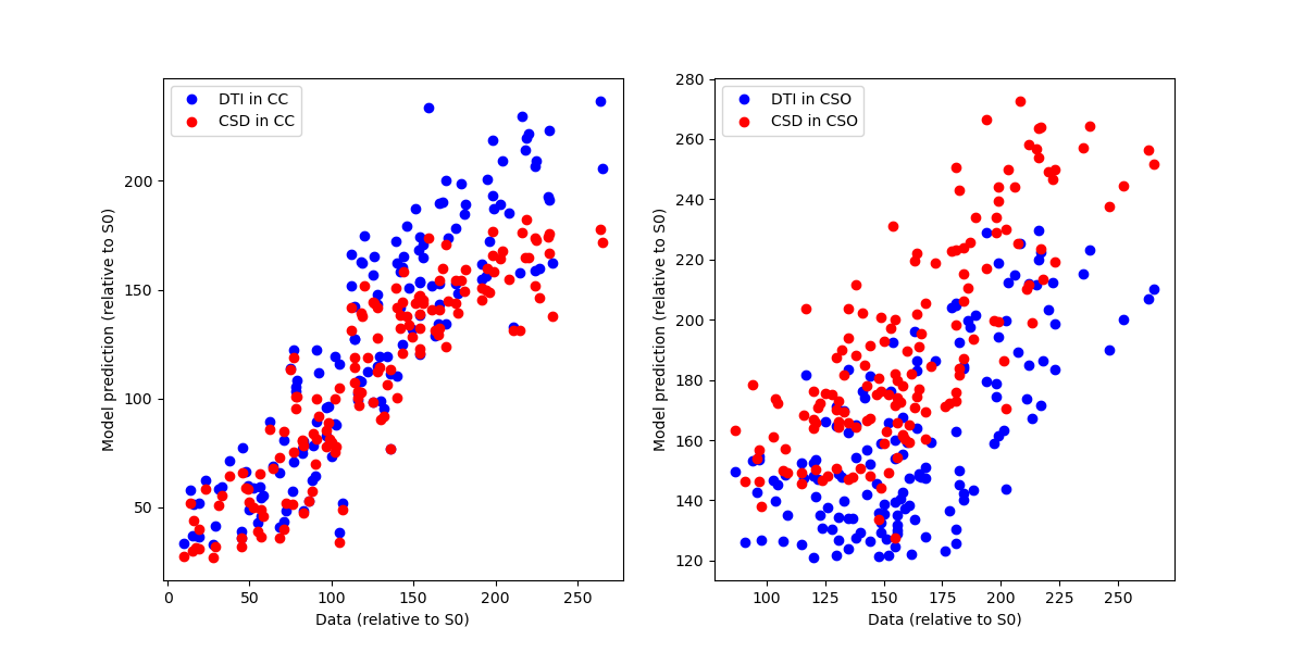
Model predictions.

We can also quantify the goodness of fit of the models by calculating an R-squared score:

cc_dti_r2 = (
    stats.pearsonr(cc_vox[gtab.b0s_mask == 0], dti_cc[gtab.b0s_mask == 0])[0] ** 2
)
cc_csd_r2 = (
    stats.pearsonr(cc_vox[gtab.b0s_mask == 0], csd_cc[gtab.b0s_mask == 0])[0] ** 2
)
cso_dti_r2 = (
    stats.pearsonr(cso_vox[gtab.b0s_mask == 0], dti_cso[gtab.b0s_mask == 0])[0] ** 2
)
cso_csd_r2 = (
    stats.pearsonr(cso_vox[gtab.b0s_mask == 0], csd_cso[gtab.b0s_mask == 0])[0] ** 2
)

print(
    "Corpus callosum\n"
    f"DTI R2 : {cc_dti_r2}\n"
    f"CSD R2 : {cc_csd_r2}\n"
    "\n"
    "Centrum Semiovale\n"
    f"DTI R2 : {cso_dti_r2}\n"
    f"CSD R2 : {cso_csd_r2}\n"
)

Corpus callosum
DTI R2 : 0.7828795917127749
CSD R2 : 0.8051656184264929

Centrum Semiovale
DTI R2 : 0.4319253628762229
CSD R2 : 0.6038698891074342

As you can see, DTI is a pretty good model for describing the signal in the CC, while CSD is much better in describing the signal in regions of multiple crossing fibers.

References

[1]

Trevor Hastie, Robert Tibshirani, and Jerome Friedman. The Elements of Statistical Learning: Data Mining, Inference, and Prediction, Second Edition. Springer, 2 edition, 2009. doi:https://doi.org/10.1007/978-0-387-84858-7.

[2]

Ariel Rokem, Kimberly L. Chan, Jason D. Yeatman, Franco Pestilli, and Brian A. Wandel. Evaluating the accuracy of diffusion models at multiple b-values with cross-validation. In Joint Annual Meeting ISMRM-ESMRMB 2014 SMRT 23rd Annual Meeting, volume. Milan, Italy, 2014. International Society for Magnetic Resonance in Medicine (ISMRM).