Note
Go to the end to download the full example code.
Reconstruction with Robust and Unbiased Model-BAsed Spherical Deconvolution (RUMBA)#
This example shows how to use RUMBA-SD to reconstruct fiber orientation density functions (fODFs). This model was introduced by Canales-Rodríguez et al.[1].
RUMBA-SD uses a priori information about the fiber response function (axial and perpendicular diffusivities) to generate a convolution kernel mapping the fODFs on a sphere to the recorded data. The fODFs are then estimated using an iterative, maximum likelihood estimation algorithm adapted from Richardson-Lucy (RL) deconvolution [2]. Specifically, the RL algorithm assumes Gaussian noise, while RUMBA assumes Rician/Noncentral Chi noise – these more accurately reflect the noise generated by MRI scanners [3]. This algorithm also contains an optional compartment for estimating an isotropic volume fraction to account for partial volume effects. RUMBA-SD works with single- and multi-shell data, as well as data recorded in Cartesian or spherical coordinate systems.
The result from RUMBA-SD can be smoothed by applying total variation spatial regularization (termed RUMBA-SD + TV), a technique which promotes a more coherent estimate of the fODFs across neighboring voxels [4]. This regularization ability is also included in this implementation.
- This example will showcase how to:
Estimate the fiber response function
Reconstruct the fODFs voxel-wise or globally with TV regularization
Visualize fODF maps
To begin, we will load the data, consisting of 10 b0s and 150 non-b0s with a b-value of 2000.
import matplotlib.pyplot as plt
import numpy as np

from dipy.core.gradients import gradient_table
from dipy.data import get_fnames, get_sphere
from dipy.direction import peak_directions, peaks_from_model
from dipy.io.gradients import read_bvals_bvecs
from dipy.io.image import load_nifti
from dipy.reconst.csdeconv import auto_response_ssst, recursive_response
from dipy.reconst.rumba import RumbaSDModel
from dipy.segment.mask import median_otsu
from dipy.sims.voxel import single_tensor_odf
from dipy.viz import actor, window

hardi_fname, hardi_bval_fname, hardi_bvec_fname = get_fnames(name="stanford_hardi")
data, affine = load_nifti(hardi_fname)

bvals, bvecs = read_bvals_bvecs(hardi_bval_fname, hardi_bvec_fname)
gtab = gradient_table(bvals, bvecs=bvecs)

sphere = get_sphere(name="symmetric362")
Step 1. Estimation of the fiber response function#
There are multiple ways to estimate the fiber response function.
Strategy 1: use default values One simple approach is to use the values included as the default arguments in the RumbaSDModel constructor. The white matter response, wm_response has three values corresponding to the tensor eigenvalues (1.7e-3, 0.2e-3, 0.2e-3). The model has compartments for cerebrospinal fluid (CSF) (csf_response) and grey matter (GM) (gm_response) as well, with these mean diffusivities set to 3.0e-3 and 0.8e-3 respectively [1] These default values will often be adequate as RUMBA-SD is robust against impulse response imprecision [5].
rumba = RumbaSDModel(gtab)
print(
    f"wm_response: {rumba.wm_response}, "
    + f"csf_response: {rumba.csf_response}, "
    + f"gm_response: {rumba.gm_response}"
)
wm_response: [0.0017 0.0002 0.0002], csf_response: 0.003, gm_response: 0.0008
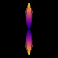
We can visualize what this default response looks like.
# Enables/disables interactive visualization
interactive = False

scene = window.Scene()

evals = rumba.wm_response
evecs = np.array([[0, 1, 0], [0, 0, 1], [1, 0, 0]]).T

response_odf = single_tensor_odf(sphere.vertices, evals=evals, evecs=evecs)
# Transform our data from 1D to 4D
response_odf = response_odf[None, None, None, :]
response_actor = actor.odf_slicer(response_odf, sphere=sphere, colormap="plasma")

scene.add(response_actor)
print("Saving illustration as default_response.png")
window.record(scene=scene, out_path="default_response.png", size=(200, 200))

if interactive:
    window.show(scene)
Saving illustration as default_response.png
Default response function.
scene.rm(response_actor)
Strategy 2: estimate from local brain region The csdeconv module contains functions for estimating this response. auto_response_sst extracts an ROI in the center of the brain and isolates single fiber populations from the corpus callosum using an FA mask with a threshold of 0.7. These voxels are used to estimate the response function.
response, _ = auto_response_ssst(gtab, data, roi_radii=10, fa_thr=0.7)
print(response)
(array([0.00139919, 0.0003007 , 0.0003007 ]), np.float64(416.7372408293461))
This response contains the estimated eigenvalues in its first element, and the estimated S0 in the second. The eigenvalues are all we care about for using RUMBA-SD.
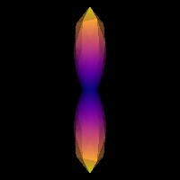
We can visualize this estimated response as well.
evals = response[0]
evecs = np.array([[0, 1, 0], [0, 0, 1], [1, 0, 0]]).T

response_odf = single_tensor_odf(sphere.vertices, evals=evals, evecs=evecs)
# transform our data from 1D to 4D
response_odf = response_odf[None, None, None, :]
response_actor = actor.odf_slicer(response_odf, sphere=sphere, colormap="plasma")
scene.add(response_actor)
print("Saving illustration as estimated_response.png")
window.record(scene=scene, out_path="estimated_response.png", size=(200, 200))
if interactive:
    window.show(scene)
Saving illustration as estimated_response.png
Estimated response function.
scene.rm(response_actor)
Strategy 3: recursive, data-driven estimation The other method for extracting a response function uses a recursive approach. Here, we initialize a “fat” response function, which is used in CSD. From this deconvolution, the voxels with one peak are extracted and their data is averaged to get a new response function. This is repeated iteratively until convergence [6].
To shorten computation time, a mask can be estimated for the data.
b0_mask, mask = median_otsu(data, median_radius=2, numpass=1, vol_idx=np.arange(10))

rec_response = recursive_response(
    gtab,
    data,
    mask=mask,
    sh_order_max=8,
    peak_thr=0.01,
    init_fa=0.08,
    init_trace=0.0021,
    iter=4,
    convergence=0.001,
    parallel=True,
    num_processes=2,
)
/Users/skoudoro/devel/dipy_wt/release/dipy/reconst/csdeconv.py:1127: RuntimeWarning: invalid value encountered in divide
  single_peak_mask = (vals[:, 1] / vals[:, 0]) < peak_thr
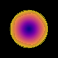
We can now visualize this response, which will look like a pancake.
rec_response_signal = rec_response.on_sphere(sphere)
# transform our data from 1D to 4D
rec_response_signal = rec_response_signal[None, None, None, :]
response_actor = actor.odf_slicer(rec_response_signal, sphere=sphere, colormap="plasma")

scene.add(response_actor)
print("Saving illustration as recursive_response.png")
window.record(scene=scene, out_path="recursive_response.png", size=(200, 200))
if interactive:
    window.show(scene)
Saving illustration as recursive_response.png
Recursive response function.
scene.rm(response_actor)
Step 2. fODF Reconstruction#
We will now use the estimated response function with the RUMBA-SD model to reconstruct the fODFs. We will use the default value for csf_response and gm_response. If one doesn’t wish to fit these compartments, one can specify either argument as None. This will result in the corresponding volume fraction map being all zeroes. The GM compartment can only be accurately estimated with at least 3-shell data. With less shells, it is recommended to only keep the compartment for CSF. Since this data is single-shell, we will only compute the CSF compartment.
RUMBA-SD can fit the data voxelwise or globally. By default, a voxelwise approach is used (voxelwise is set to True). However, by setting voxelwise to false, the whole brain can be fit at once. In this global setting, one can specify the use of TV regularization with use_tv, and the model can log updates on its progress and estimated signal-to-noise ratios by setting verbose to True. By default, both use_tv and verbose are set to False as they have no bearing on the voxelwise fit.
When constructing the RUMBA-SD model, one can also specify n_iter, recon_type, n_coils, R, and sphere. n_iter is the number of iterations for the iterative estimation, and the default value of 600 should be suitable for most applications. recon_type is the technique used by the MRI scanner to reconstruct the MRI signal, and should be either ‘smf’ for ‘spatial matched filter’, or ‘sos’ for ‘sum-of-squares’; ‘smf’ is a common choice and is the default, but the specifications of the MRI scanner used to collect the data should be checked. If ‘sos’ is used, then it’s important to specify n_coils, which is the number of coils in the MRI scanner. With ‘smf’, this isn’t important and the default argument of 1 can be used. R is the acceleration factor of the MRI scanner, which is termed the iPAT factor for SIEMENS, the ASSET factor for GE, or the SENSE factor for PHILIPS. 1 is a common choice, and is the default for the model. This is only important when using TV regularization, which will be covered later in the tutorial. Finally, sphere specifies the sphere on which to construct the fODF. The default is ‘repulsion724’ sphere, but this tutorial will use symmetric362.
For efficiency, we will only fit a small part of the data. This is the same portion of data used in Reconstruction with Constrained Spherical Deconvolution model (CSD).
data_small = data[20:50, 55:85, 38:39]
Option 1: voxel-wise fit This is the default approach for generating ODFs, wherein each voxel is fit sequentially.
We will estimate the fODFs using the ‘symmetric362’ sphere. This will take about a minute to compute.
rumba_fit = rumba.fit(data_small)
odf = rumba_fit.odf()
The inclusion of RUMBA-SD’s CSF compartment means we can also extract the isotropic volume fraction map as well as the white matter volume fraction map (the fODF sum at each voxel). These values are normalized such that they sum to 1. If neither isotropic compartment is included, then the isotropic volume fraction map will all be zeroes.
We can visualize these maps using adjacent heatmaps.
fig, axs = plt.subplots(1, 2, figsize=(12, 5))

ax0 = axs[0].imshow(f_wm[..., 0].T, origin="lower")
axs[0].set_title("Voxelwise White Matter Volume Fraction")

ax1 = axs[1].imshow(f_iso[..., 0].T, origin="lower")
axs[1].set_title("Voxelwise Isotropic Volume Fraction")

plt.colorbar(ax0, ax=axs[0])
plt.colorbar(ax1, ax=axs[1])

plt.savefig("wm_iso_partition.png")
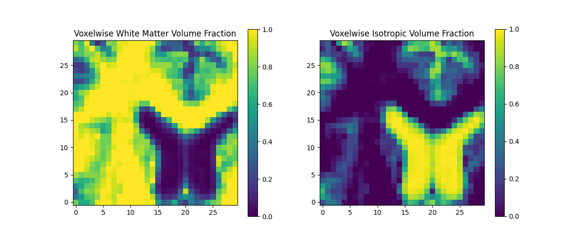
White matter and isotropic volume fractions
To visualize the fODFs, it’s recommended to combine the fODF and the isotropic components. This is done using the RumbaFit object’s method combined_odf_iso. To reach a proper scale for visualization, the argument norm=True is used in FURY’s odf_slicer method.
combined = rumba_fit.combined_odf_iso

fodf_spheres = actor.odf_slicer(
    combined, sphere=sphere, norm=True, scale=0.5, colormap=None
)
scene.add(fodf_spheres)
print("Saving illustration as rumba_odfs.png")
window.record(scene=scene, out_path="rumba_odfs.png", size=(600, 600))
if interactive:
    window.show(scene)
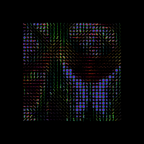
Saving illustration as rumba_odfs.png
RUMBA-SD fODFs
scene.rm(fodf_spheres)
We can extract the peaks from these fODFs using peaks_from_model. This will reconstruct the fODFs again, so will take about a minute to run.
For visualization, we scale up the peak values.
peak_values = np.clip(rumba_peaks.peak_values * 15, 0, 1)
peak_dirs = rumba_peaks.peak_dirs

fodf_peaks = actor.peak_slicer(peak_dirs, peaks_values=peak_values)
scene.add(fodf_peaks)

window.record(scene=scene, out_path="rumba_peaks.png", size=(600, 600))
if interactive:
    window.show(scene)
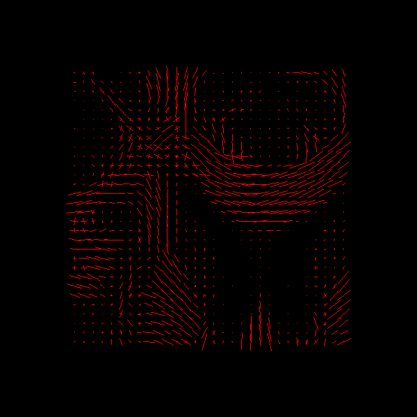
RUMBA-SD peaks
scene.rm(fodf_peaks)
Option 2: global fit Instead of the voxel-wise fit, RUMBA also comes with an implementation of global fitting where all voxels are fit simultaneously. This comes with some potential benefits such as:
More efficient fitting due to matrix parallelization, in exchange for larger demands on RAM (>= 16 GB should be sufficient)
The option for spatial regularization; specifically, TV regularization is built into the fitting function (RUMBA-SD + TV)
This is done by setting voxelwise to False, and setting use_tv to True.
TV regularization requires a volume without any singleton dimensions, so we’ll have to start by expanding our data slice.
Now, we fit the model in the same way. This will take about 90 seconds.
rumba_fit = rumba.fit(data_tv)

odf = rumba_fit.odf()
combined = rumba_fit.combined_odf_iso
Now we can visualize the combined fODF map as before.
fodf_spheres = actor.odf_slicer(
    combined, sphere=sphere, norm=True, scale=0.5, colormap=None
)

scene.add(fodf_spheres)
print("Saving illustration as rumba_global_odfs.png")
window.record(scene=scene, out_path="rumba_global_odfs.png", size=(600, 600))
if interactive:
    window.show(scene)
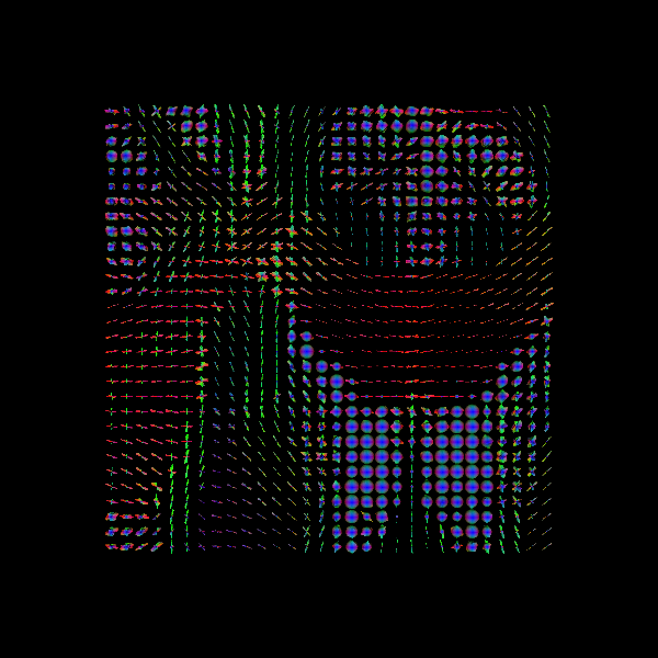
Saving illustration as rumba_global_odfs.png
RUMBA-SD + TV fODFs
This can be compared with the result without TV regularization, and one can observe that the coherence between neighboring voxels is improved.
scene.rm(fodf_spheres)
For peak detection, peaks_from_model cannot be used as it doesn’t support global fitting approaches. Instead, we’ll compute our peaks using a for loop.
shape = odf.shape[:3]
npeaks = 5  # maximum number of peaks returned for a given voxel
peak_dirs = np.zeros((shape + (npeaks, 3)))
peak_values = np.zeros((shape + (npeaks,)))

for idx in np.ndindex(shape):  # iterate through each voxel
    # Get peaks of odf
    direction, pk, _ = peak_directions(
        odf[idx], sphere, relative_peak_threshold=0.5, min_separation_angle=25
    )

    # Calculate peak metrics
    if pk.shape[0] != 0:
        n = min(npeaks, pk.shape[0])
        peak_dirs[idx][:n] = direction[:n]
        peak_values[idx][:n] = pk[:n]

# Scale up for visualization
peak_values = np.clip(peak_values * 15, 0, 1)

fodf_peaks = actor.peak_slicer(
    peak_dirs[:, :, 0:1, :], peaks_values=peak_values[:, :, 0:1, :]
)
scene.add(fodf_peaks)

print("Saving illustration as rumba_global_peaks.png")
window.record(scene=scene, out_path="rumba_global_peaks.png", size=(600, 600))
if interactive:
    window.show(scene)
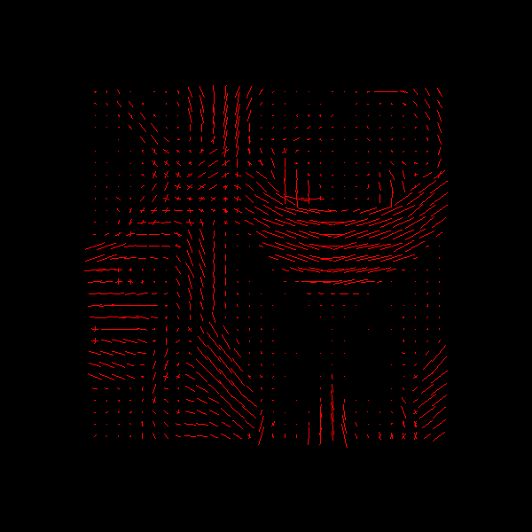
Saving illustration as rumba_global_peaks.png
RUMBA-SD + TV peaks
scene.rm(fodf_peaks)
References#
Total running time of the script: (3 minutes 39.594 seconds)