Note
Go to the end to download the full example code.
Estimating diffusion time dependent q-space indices using qt-dMRI#
Effective representation of the four-dimensional diffusion MRI signal – varying over three-dimensional q-space and diffusion time – is a sought-after and still unsolved challenge in diffusion MRI (dMRI). We propose a functional basis approach that is specifically designed to represent the dMRI signal in this qtau-space [1]. Following recent terminology, we refer to our qtau-functional basis as \(q au\)-dMRI. We use GraphNet regularization –imposing both signal smoothness and sparsity – to drastically reduce the number of diffusion-weighted images (DWIs) that is needed to represent the dMRI signal in the qtau-space. As the main contribution, \(q au\)-dMRI provides the framework to – without making biophysical assumptions – represent the \(q au\)-space signal and estimate time-dependent q-space indices (\(q au\)-indices), providing a new means for studying diffusion in nervous tissue. \(q au\)-dMRI is the first of its kind in being specifically designed to provide open interpretation of the \(q au\)-diffusion signal.
\(q au\)-dMRI can be seen as a time-dependent extension of the MAP-MRI functional basis [2], and all the previously proposed q-space can be estimated for any diffusion time. These include rotationally invariant quantities such as the Mean Squared Displacement (MSD), Q-space Inverse Variance (QIV) and Return-To-Origin Probability (RTOP). Also directional indices such as the Return To the Axis Probability (RTAP) and Return To the Plane Probability (RTPP) are available, as well as the Orientation Distribution Function (ODF).
In this example we illustrate how to use the \(q au\)-dMRI to estimate time-dependent q-space indices from a \(q au\)-acquisition of a mouse.
First import the necessary modules:
import matplotlib.pyplot as plt
import numpy as np

from dipy.data.fetcher import (
    fetch_qtdMRI_test_retest_2subjects,
    read_qtdMRI_test_retest_2subjects,
)
from dipy.reconst import dti, qtdmri
Download and read the data for this tutorial.
\(q\tau\)-dMRI requires data with multiple gradient directions, gradient strength and diffusion times. We will use the test-retest acquisitions of two mice that were used in the test-retest study by [1]. The data itself is freely available and citeable at [3].
data contains 4 qt-dMRI datasets of size [80, 160, 5, 515]. The first two are the test-retest datasets of the first mouse and the second two are those of the second mouse. cc_masks contains 4 corresponding binary masks for the corpus callosum voxels in the middle slice that were used in the test-retest study. Finally, gtab contains the qt-dMRI gradient tables for the DWIs in the dataset.
The data consists of 515 DWIs, divided over 35 shells, with 7 “gradient strength shells” up to 491 mT/m, 5 equally spaced “pulse separation shells” (big_delta) between [10.8-20] ms and a pulse duration (small_delta) of 5ms.
To visualize qt-dMRI acquisition schemes in an intuitive way, the qtdmri module provides a visualization function to illustrate the relationship between gradient strength (G), pulse separation (big_delta) and b-value:
plt.figure()
qtdmri.visualise_gradient_table_G_Delta_rainbow(gtabs[0])
plt.savefig("qt-dMRI_acquisition_scheme.png")
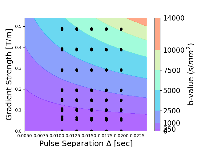
In the figure the dots represent measured DWIs in any direction, for a given gradient strength and pulse separation. The background isolines represent the corresponding b-values for different combinations of G and big_delta.
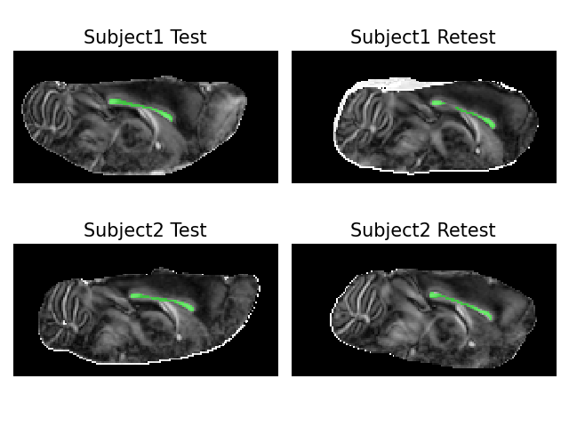
Next, we visualize the middle slices of the test-retest data sets with their corresponding masks. To better illustrate the white matter architecture in the data, we calculate DTI’s fractional anisotropy (FA) over the whole slice and project the corpus callosum mask on the FA image.:
subplot_titles = [
    "Subject1 Test",
    "Subject1 Retest",
    "Subject2 Test",
    "Subject2 Retest",
]
fig = plt.figure()
plt.subplots(nrows=2, ncols=2)
for i, (data_, mask_, gtab_) in enumerate(zip(data, cc_masks, gtabs)):
    # take the middle slice
    data_middle_slice = data_[:, :, 2]
    mask_middle_slice = mask_[:, :, 2]

    # estimate fractional anisotropy (FA) for this slice
    tenmod = dti.TensorModel(gtab_)
    tenfit = tenmod.fit(data_middle_slice, mask=data_middle_slice[..., 0] > 0)
    fa = tenfit.fa

    # set mask color to green with 0.5 opacity as overlay
    mask_template = np.zeros(np.r_[mask_middle_slice.shape, 4])
    mask_template[mask_middle_slice == 1] = np.r_[0.0, 1.0, 0.0, 0.5]

    # produce the FA images with corpus callosum masks.
    plt.subplot(2, 2, 1 + i)
    plt.title(subplot_titles[i], fontsize=15)
    plt.imshow(fa, cmap="Greys_r", origin="lower", interpolation="nearest")
    plt.imshow(mask_template, origin="lower", interpolation="nearest")
    plt.axis("off")
plt.tight_layout()
plt.savefig("qt-dMRI_datasets_fa_with_ccmasks.png")
Next, we use qt-dMRI to estimate of time-dependent q-space indices (q:math:tau-indices) for the masked voxels in the corpus callosum of each dataset. In particular, we estimate the Return-to-Original, Return-to-Axis and Return-to-Plane Probability (RTOP, RTAP and RTPP), as well as the Mean Squared Displacement (MSD).
In this example we don’t extrapolate the data beyond the maximum diffusion time, so we estimate \(q\tau\) indices between the minimum and maximum diffusion times of the data at 5 equally spaced points. However, it should the noted that qt-dMRI’s combined smoothness and sparsity regularization allows for smooth interpolation at any \(q\tau\) position. In other words, once the basis is fitted to the data, its coefficients describe the entire \(q\tau\)-space, and any \(q\tau\)-position can be freely recovered. This including points beyond the dataset’s maximum \(q\tau\) value (although this should be done with caution).
tau_min = gtabs[0].tau.min()
tau_max = gtabs[0].tau.max()
taus = np.linspace(tau_min, tau_max, 5)

qtdmri_fits = []
msds = []
rtops = []
rtaps = []
rtpps = []
for data_, mask_, gtab_ in zip(data, cc_masks, gtabs):
    # select the corpus callosum voxel for every dataset
    cc_voxels = data_[mask_ == 1]
    # initialize the qt-dMRI model.
    # recommended basis orders are radial_order=6 and time_order=2.
    # The combined Laplacian and l1-regularization using Generalized
    # Cross-Validation (GCV) and Cross-Validation (CV) settings is most robust,
    # but can be used separately and with weightings preset to any positive
    # value to optimize for speed.
    qtdmri_mod = qtdmri.QtdmriModel(
        gtab_,
        radial_order=6,
        time_order=2,
        laplacian_regularization=True,
        laplacian_weighting="GCV",
        l1_regularization=True,
        l1_weighting="CV",
    )
    # fit the model.
    # Here we take every 5th voxel for speed, but of course all voxels can be
    # fit for a more robust result later on.
    qtdmri_fit = qtdmri_mod.fit(cc_voxels[::5])
    qtdmri_fits.append(qtdmri_fit)
    # We estimate MSD, RTOP, RTAP and RTPP for the chosen diffusion times.
    msds.append(np.array(list(map(qtdmri_fit.msd, taus))))
    rtops.append(np.array(list(map(qtdmri_fit.rtop, taus))))
    rtaps.append(np.array(list(map(qtdmri_fit.rtap, taus))))
    rtpps.append(np.array(list(map(qtdmri_fit.rtpp, taus))))
The estimated \(q\tau\)-indices, for the chosen diffusion times, are now stored in msds, rtops, rtaps and rtpps. The trends of these \(q\tau\)-indices over time say something about the restriction of diffusing particles over time, which is currently a hot topic in the dMRI community. We evaluate the test-retest reproducibility for the two subjects by plotting the \(q\tau\)-indices for each subject together. This example will produce similar results as Fig. 10 in [1].
We first define a small function to plot the mean and standard deviation of the \(q\tau\)-index trends in a subject.
def plot_mean_with_std(ax, time, ind1, plotcolor, ls="-", std_mult=1, label=""):
    means = np.mean(ind1, axis=1)
    stds = np.std(ind1, axis=1)
    ax.plot(time, means, c=plotcolor, lw=3, label=label, ls=ls)
    ax.fill_between(
        time,
        means + std_mult * stds,
        means - std_mult * stds,
        alpha=0.15,
        color=plotcolor,
    )
    ax.plot(time, means + std_mult * stds, alpha=0.25, color=plotcolor)
    ax.plot(time, means - std_mult * stds, alpha=0.25, color=plotcolor)
We start by showing the test-retest MSD of both subjects over time. We plot the \(q\tau\)-indices together with \(q\tau\)-index trends of free diffusion with different diffusivities as background.
# we first generate the data to produce the background index isolines.
Delta_ = np.linspace(0.005, 0.02, 100)
MSD_ = np.linspace(4e-5, 10e-5, 100)
Delta_grid, MSD_grid = np.meshgrid(Delta_, MSD_)
D_grid = MSD_grid / (6 * Delta_grid)
D_levels = np.r_[1, 5, 7, 10, 14, 23, 30] * 1e-4

fig = plt.figure(figsize=(10, 3))
# start with the plot of subject 1.
ax = plt.subplot(1, 2, 1)
# first plot the background
plt.contourf(Delta_ * 1e3, 1e5 * MSD_, D_grid, levels=D_levels, cmap="Greys", alpha=0.5)

# plot the test-retest mean MSD and standard deviation of subject 1.
plot_mean_with_std(ax, taus * 1e3, 1e5 * msds[0], "r", "dashdot", label="MSD Test")
plot_mean_with_std(ax, taus * 1e3, 1e5 * msds[1], "g", "dashdot", label="MSD Retest")
ax.legend(fontsize=13)
# plot some text markers to clarify the background diffusivity lines.
ax.text(0.0091 * 1e3, 6.33, "D=14e-4", fontsize=12, rotation=35)
ax.text(0.0091 * 1e3, 4.55, "D=10e-4", fontsize=12, rotation=25)
ax.set_ylim(4, 9.5)
ax.set_xlim(0.009 * 1e3, 0.0185 * 1e3)
ax.set_title(r"Test-Retest MSD(:math:`\tau`) Subject 1", fontsize=15)
ax.set_xlabel("Diffusion Time (ms)", fontsize=17)
ax.set_ylabel("MSD (:math:`10^{-5}mm^2`)", fontsize=17)

# then do the same thing for subject 2.
ax = plt.subplot(1, 2, 2)
plt.contourf(Delta_ * 1e3, 1e5 * MSD_, D_grid, levels=D_levels, cmap="Greys", alpha=0.5)
cb = plt.colorbar()
cb.set_label("Free Diffusivity (:math:`mm^2/s`)", fontsize=18)

plot_mean_with_std(ax, taus * 1e3, 1e5 * msds[2], "r", "dashdot")
plot_mean_with_std(ax, taus * 1e3, 1e5 * msds[3], "g", "dashdot")
ax.set_ylim(4, 9.5)
ax.set_xlim(0.009 * 1e3, 0.0185 * 1e3)
ax.set_xlabel("Diffusion Time (ms)", fontsize=17)
ax.set_title(r"Test-Retest MSD(:math:`\tau`) Subject 2", fontsize=15)
plt.savefig("qt_indices_msd.png")
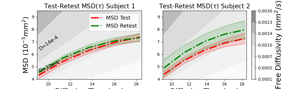
You can see that the MSD in both subjects increases over time, but also slowly levels off as time progresses. This makes sense as diffusing particles are becoming more restricted by surrounding tissue as time goes on. You can also see that for Subject 1 the index trends nearly perfectly overlap, but for subject 2 they are slightly off, which is also what we found in the paper.
Next, we follow the same procedure to estimate the test-retest RTAP, RTOP and RTPP over diffusion time for both subject. For ease of comparison, we will estimate all three in the same unit [1/mm] by taking the square root of RTAP and the cubed root of RTOP.
# Again, first we define the data for the background illustration.
Delta_ = np.linspace(0.005, 0.02, 100)
RTXP_ = np.linspace(1, 200, 100)
Delta_grid, RTXP_grid = np.meshgrid(Delta_, RTXP_)
D_grid = 1 / (4 * RTXP_grid**2 * np.pi * Delta_grid)
D_levels = np.r_[1, 2, 3, 4, 6, 9, 15, 30] * 1e-4
D_colors = np.tile(np.linspace(0.8, 0, 7), (3, 1)).T

# We start with estimating the RTOP illustration.
fig = plt.figure(figsize=(10, 3))
ax = plt.subplot(1, 2, 1)
plt.contourf(Delta_ * 1e3, RTXP_, D_grid, colors=D_colors, levels=D_levels, alpha=0.5)

plot_mean_with_std(
    ax, taus * 1e3, rtops[0] ** (1 / 3.0), "r", "--", label="RTOP:math:`^{1/3}` Test"
)
plot_mean_with_std(
    ax, taus * 1e3, rtops[1] ** (1 / 3.0), "g", "--", label="RTOP:math:`^{1/3}` Retest"
)
ax.legend(fontsize=13)
ax.text(0.0091 * 1e3, 162, "D=3e-4", fontsize=12, rotation=-22)
ax.text(0.0091 * 1e3, 140, "D=4e-4", fontsize=12, rotation=-20)
ax.text(0.0091 * 1e3, 113, "D=6e-4", fontsize=12, rotation=-16)
ax.set_ylim(54, 170)
ax.set_xlim(0.009 * 1e3, 0.0185 * 1e3)
ax.set_title(r"Test-Retest RTOP(:math:`\tau`) Subject 1", fontsize=15)
ax.set_xlabel("Diffusion Time (ms)", fontsize=17)
ax.set_ylabel("RTOP:math:`^{1/3}` (1/mm)", fontsize=17)

ax = plt.subplot(1, 2, 2)
plt.contourf(Delta_ * 1e3, RTXP_, D_grid, colors=D_colors, levels=D_levels, alpha=0.5)
cb = plt.colorbar()
cb.set_label("Free Diffusivity (:math:`mm^2/s`)", fontsize=18)

plot_mean_with_std(ax, taus * 1e3, rtops[2] ** (1 / 3.0), "r", "--")
plot_mean_with_std(ax, taus * 1e3, rtops[3] ** (1 / 3.0), "g", "--")
ax.set_ylim(54, 170)
ax.set_xlim(0.009 * 1e3, 0.0185 * 1e3)
ax.set_xlabel("Diffusion Time (ms)", fontsize=17)
ax.set_title(r"Test-Retest RTOP(:math:`\tau`) Subject 2", fontsize=15)
plt.savefig("qt_indices_rtop.png")
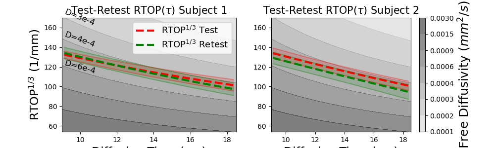
Similarly as MSD, the RTOP is related to the restriction that particles are experiencing and is also rotationally invariant. RTOP is defined as the probability that particles are found at the same position at the time of both gradient pulses. As time increases, the odds become smaller that a particle will arrive at the same position it left, which is illustrated by all RTOP trends in the figure. Notice that the estimated RTOP trends decrease less fast than free diffusion, meaning that particles experience restriction over time. Also notice that the RTOP trends in both subjects nearly perfectly overlap.
Next, we estimate two directional \(q\tau\)-indices, RTAP and RTPP, describing particle restriction perpendicular and parallel to the orientation of the principal diffusivity in that voxel. If the voxel describes coherent white matter (which it does in our corpus callosum example), then they describe properties related to restriction perpendicular and parallel to the axon bundles.
# First, we estimate the RTAP trends.
fig = plt.figure(figsize=(10, 3))
ax = plt.subplot(1, 2, 1)
plt.contourf(Delta_ * 1e3, RTXP_, D_grid, colors=D_colors, levels=D_levels, alpha=0.5)

plot_mean_with_std(
    ax, taus * 1e3, np.sqrt(rtaps[0]), "r", "-", label="RTAP:math:`^{1/2}` Test"
)
plot_mean_with_std(
    ax, taus * 1e3, np.sqrt(rtaps[1]), "g", "-", label="RTAP:math:`^{1/2}` Retest"
)
ax.legend(fontsize=13)
ax.text(0.0091 * 1e3, 162, "D=3e-4", fontsize=12, rotation=-22)
ax.text(0.0091 * 1e3, 140, "D=4e-4", fontsize=12, rotation=-20)
ax.text(0.0091 * 1e3, 113, "D=6e-4", fontsize=12, rotation=-16)
ax.set_ylim(54, 170)
ax.set_xlim(0.009 * 1e3, 0.0185 * 1e3)
ax.set_title(r"Test-Retest RTAP(:math:`\tau`) Subject 1", fontsize=15)
ax.set_xlabel("Diffusion Time (ms)", fontsize=17)
ax.set_ylabel("RTAP:math:`^{1/2}` (1/mm)", fontsize=17)

ax = plt.subplot(1, 2, 2)
plt.contourf(Delta_ * 1e3, RTXP_, D_grid, colors=D_colors, levels=D_levels, alpha=0.5)
cb = plt.colorbar()
cb.set_label("Free Diffusivity (:math:`mm^2/s`)", fontsize=18)

plot_mean_with_std(ax, taus * 1e3, np.sqrt(rtaps[2]), "r", "-")
plot_mean_with_std(ax, taus * 1e3, np.sqrt(rtaps[3]), "g", "-")
ax.set_ylim(54, 170)
ax.set_xlim(0.009 * 1e3, 0.0185 * 1e3)
ax.set_xlabel("Diffusion Time (ms)", fontsize=17)
ax.set_title(r"Test-Retest RTAP(:math:`\tau`) Subject 2", fontsize=15)
plt.savefig("qt_indices_rtap.png")


# Finally the last one for RTPP.
fig = plt.figure(figsize=(10, 3))
ax = plt.subplot(1, 2, 1)
plt.contourf(Delta_ * 1e3, RTXP_, D_grid, colors=D_colors, levels=D_levels, alpha=0.5)

plot_mean_with_std(ax, taus * 1e3, rtpps[0], "r", ":", label="RTPP Test")
plot_mean_with_std(ax, taus * 1e3, rtpps[1], "g", ":", label="RTPP Retest")
ax.legend(fontsize=13)
ax.text(0.0091 * 1e3, 113, "D=6e-4", fontsize=12, rotation=-16)
ax.text(0.0091 * 1e3, 91, "D=9e-4", fontsize=12, rotation=-13)
ax.text(0.0091 * 1e3, 69, "D=15e-4", fontsize=12, rotation=-10)
ax.set_ylim(54, 170)
ax.set_xlim(0.009 * 1e3, 0.0185 * 1e3)
ax.set_title(r"Test-Retest RTPP(:math:`\tau`) Subject 1", fontsize=15)
ax.set_xlabel("Diffusion Time (ms)", fontsize=17)
ax.set_ylabel("RTPP (1/mm)", fontsize=17)

ax = plt.subplot(1, 2, 2)
plt.contourf(Delta_ * 1e3, RTXP_, D_grid, colors=D_colors, levels=D_levels, alpha=0.5)
cb = plt.colorbar()
cb.set_label("Free Diffusivity (:math:`mm^2/s`)", fontsize=18)

plot_mean_with_std(ax, taus * 1e3, rtpps[2], "r", ":")
plot_mean_with_std(ax, taus * 1e3, rtpps[3], "g", ":")
ax.set_ylim(54, 170)
ax.set_xlim(0.009 * 1e3, 0.0185 * 1e3)
ax.set_xlabel("Diffusion Time (ms)", fontsize=17)
ax.set_title(r"Test-Retest RTPP(:math:`\tau`) Subject 2", fontsize=15)
plt.savefig("qt_indices_rtpp.png")
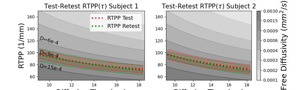
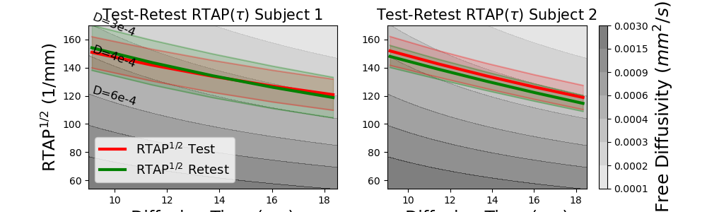
As those of RTOP, the trends in RTAP and RTPP also decrease over time. It can be seen that RTAP:math:^{1/2} is always bigger than RTPP, which makes sense as particles in coherent white matter experience more restriction perpendicular to the white matter orientation than parallel to it. Again, in both subjects the test-retest RTAP and RTPP is nearly perfectly consistent. Aside from the estimation of \(q\tau\)-space indices, \(q\tau\)-dMRI also allows for the estimation of time-dependent ODFs. Once the Qtdmri model is fitted it can be simply called by qtdmri_fit.odf(sphere, s=sharpening_factor). This is identical to how the mapmri module functions, and allows one to study the time-dependence of ODF directionality.
This concludes the example on qt-dMRI. As we showed, approaches such as qt-dMRI can help in studying the (finite-\(\tau\)) temporal properties of diffusion in biological tissues. Differences in \(q\tau\)-index trends could be indicative of underlying structural differences that affect the time-dependence of the diffusion process.
References#
Total running time of the script: (3 minutes 46.247 seconds)