Extracting AFQ tract profiles from segmented bundles

In this example, we will extract the values of a statistic from a volume, using the coordinates along the length of a bundle. These are called tract profiles

One of the challenges of extracting tract profiles is that some of the streamlines in a bundle may diverge significantly from the bundle in some locations. To overcome this challenge, we will use a strategy similar to that described in [Yeatman2012]: We will weight the contribution of each streamline to the bundle profile based on how far this streamline is from the mean trajectory of the bundle at that location.

import dipy.stats.analysis as dsa
import dipy.tracking.streamline as dts
from dipy.segment.clustering import QuickBundles
from dipy.segment.metricspeed import AveragePointwiseEuclideanMetric
from dipy.segment.featurespeed import ResampleFeature
from dipy.data.fetcher import get_two_hcp842_bundles
import dipy.data as dpd
from dipy.io.streamline import load_trk
from dipy.io.image import load_nifti
import matplotlib.pyplot as plt
import numpy as np
import os.path as op

To get started, we will grab the bundles.

bundles_path = dpd.fetch_bundles_2_subjects()
bundles_folder = bundles_path[1]

cst_l_file = op.join(bundles_folder, "bundles_2_subjects", "subj_2", "bundles",
                     "bundles_cst.left.trk")
af_l_file = op.join(bundles_folder, "bundles_2_subjects", "subj_2", "bundles",
                    "bundles_af.left.trk")

Either way, we can use the dipy.io API to read in the bundles from file. load_trk returns both the streamlines, as well as header information.

cst_l = load_trk(cst_l_file, "same", bbox_valid_check=False).streamlines
af_l = load_trk(af_l_file, "same", bbox_valid_check=False).streamlines

In the next step, we need to make sure that all the streamlines in each bundle are oriented the same way. For example, for the CST, we want to make sure that all the bundles have their cortical termination at one end of the streamline. This is that when we later extract values from a volume, we won’t have different streamlines going in opposite directions.

To orient all the streamlines in each bundles, we will create standard streamlines, by finding the centroids of the left AF and CST bundle models.

The advantage of using the model bundles is that we can use the same standard for different subjects, which means that we’ll get roughly the same orientation

model_af_l_file, model_cst_l_file = get_two_hcp842_bundles()

model_af_l = load_trk(model_af_l_file, "same",
                      bbox_valid_check=False).streamlines
model_cst_l = load_trk(model_cst_l_file, "same",
                       bbox_valid_check=False).streamlines


feature = ResampleFeature(nb_points=100)
metric = AveragePointwiseEuclideanMetric(feature)

Since we are going to include all of the streamlines in the single cluster from the streamlines, we set the threshold to np.inf. We pull out the centroid as the standard.

qb = QuickBundles(np.inf, metric=metric)

cluster_cst_l = qb.cluster(model_cst_l)
standard_cst_l = cluster_cst_l.centroids[0]

cluster_af_l = qb.cluster(model_af_l)
standard_af_l = cluster_af_l.centroids[0]

We use the centroid streamline for each atlas bundle as the standard to orient all of the streamlines in each bundle from the individual subject. Here, the affine used is the one from the transform between the atlas and individual tractogram. This is so that the orienting is done relative to the space of the individual, and not relative to the atlas space.

oriented_cst_l = dts.orient_by_streamline(cst_l, standard_cst_l)
oriented_af_l = dts.orient_by_streamline(af_l, standard_af_l)

Read volumetric data from an image corresponding to this subject.

For the purpose of this, we’ve extracted only the FA within the bundles in question, but in real use, this is where you would add the FA map of your subject.

files, folder = dpd.fetch_bundle_fa_hcp()

fa, fa_affine = load_nifti(op.join(folder, "hcp_bundle_fa.nii.gz"))

Calculate weights for each bundle:

w_cst_l = dsa.gaussian_weights(oriented_cst_l)
w_af_l = dsa.gaussian_weights(oriented_af_l)

And then use the weights to calculate the tract profiles for each bundle

profile_cst_l = dsa.afq_profile(fa, oriented_cst_l, fa_affine,
                                weights=w_cst_l)

profile_af_l = dsa.afq_profile(fa, oriented_af_l, fa_affine,
                               weights=w_af_l)

fig, (ax1, ax2) = plt.subplots(1, 2)

ax1.plot(profile_cst_l)
ax1.set_ylabel("Fractional anisotropy")
ax1.set_xlabel("Node along CST")
ax2.plot(profile_af_l)
ax2.set_xlabel("Node along AF")
fig.savefig("tract_profiles")

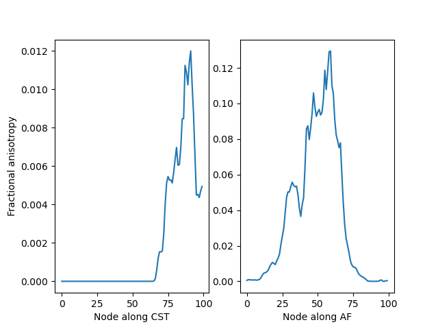
Bundle profiles for the fractional anisotropy in the left CST (left) and left AF (right).

References

[Yeatman2012]

Yeatman, Jason D., Robert F. Dougherty, Nathaniel J. Myall, Brian A. Wandell, and Heidi M. Feldman. 2012. “Tract Profiles of White Matter Properties: Automating Fiber-Tract Quantification” PloS One 7 (11): e49790.

[Garyfallidis17]

Garyfallidis et al. Recognition of white matter bundles using local and global streamline-based registration and clustering, Neuroimage, 2017.

[Garyfallidis12]

Garyfallidis E. et al., QuickBundles a method for tractography simplification, Frontiers in Neuroscience, vol 6, no 175, 2012.