Getting started with DIPY

In diffusion MRI (dMRI) usually we use three types of files, a Nifti file with the diffusion weighted data, and two text files one with b-values and one with the b-vectors.

In DIPY we provide tools to load and process these files and we also provide access to publicly available datasets for those who haven’t acquired yet their own datasets.

Let’s start with some necessary imports.

from os.path import expanduser, join

import matplotlib.pyplot as plt

from dipy.core.gradients import gradient_table
from dipy.data import fetch_sherbrooke_3shell
from dipy.io import read_bvals_bvecs
from dipy.io.image import load_nifti, save_nifti

With the following commands we can download a dMRI dataset

fetch_sherbrooke_3shell()

({'HARDI193.nii.gz': ('https://digital.lib.washington.edu/researchworks/bitstream/handle/1773/38475/HARDI193.nii.gz', '0b735e8f16695a37bfbd66aab136eb66'), 'HARDI193.bval': ('https://digital.lib.washington.edu/researchworks/bitstream/handle/1773/38475/HARDI193.bval', 'e9b9bb56252503ea49d31fb30a0ac637'), 'HARDI193.bvec': ('https://digital.lib.washington.edu/researchworks/bitstream/handle/1773/38475/HARDI193.bvec', '0c83f7e8b917cd677ad58a078658ebb7')}, 'C:\\Users\\skoudoro\\.dipy\\sherbrooke_3shell')

By default these datasets will go in the .dipy folder inside your home directory. Here is how you can access them.

home = expanduser('~')

dname holds the directory name where the 3 files are in.

dname = join(home, '.dipy', 'sherbrooke_3shell')

Here, we show the complete filenames of the 3 files

fdwi = join(dname, 'HARDI193.nii.gz')

print(fdwi)

fbval = join(dname, 'HARDI193.bval')

print(fbval)

fbvec = join(dname, 'HARDI193.bvec')

print(fbvec)

C:\Users\skoudoro\.dipy\sherbrooke_3shell\HARDI193.nii.gz
C:\Users\skoudoro\.dipy\sherbrooke_3shell\HARDI193.bval
C:\Users\skoudoro\.dipy\sherbrooke_3shell\HARDI193.bvec

Now, that we have their filenames we can start checking what these look like.

Let’s start first by loading the dMRI datasets. For this purpose, we use a python library called nibabel which enables us to read and write neuroimaging-specific file formats.

data, affine, img = load_nifti(fdwi, return_img=True)

data is a 4D array where the first 3 dimensions are the i, j, k voxel coordinates and the last dimension is the number of non-weighted (S0s) and diffusion-weighted volumes.

We can very easily check the size of data in the following way:

print(data.shape)

(128, 128, 60, 193)

We can also check the dimensions of each voxel in the following way:

print(img.header.get_zooms()[:3])

(2.0, 2.0, 2.0)

We can quickly visualize the results using matplotlib. For example, let’s show here the middle axial slices of volume 0 and volume 10.

axial_middle = data.shape[2] // 2
plt.figure('Showing the datasets')
plt.subplot(1, 2, 1).set_axis_off()
plt.imshow(data[:, :, axial_middle, 0].T, cmap='gray', origin='lower')
plt.subplot(1, 2, 2).set_axis_off()
plt.imshow(data[:, :, axial_middle, 10].T, cmap='gray', origin='lower')
plt.show()
plt.savefig('data.png', bbox_inches='tight')

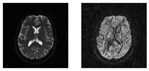
Showing the middle axial slice without (left) and with (right) diffusion weighting.

The next step is to load the b-values and b-vectors from the disk using the function read_bvals_bvecs.

bvals, bvecs = read_bvals_bvecs(fbval, fbvec)

In DIPY, we use an object called GradientTable which holds all the acquisition specific parameters, e.g. b-values, b-vectors, timings and others. To create this object you can use the function gradient_table.

gtab = gradient_table(bvals, bvecs)

Finally, you can use gtab (the GradientTable object) to show some information about the acquisition parameters

print(gtab.info)

B-values shape (193,)
         min 0.000000
         max 3500.000000
B-vectors shape (193, 3)
          min -0.964050
          max 0.999992

None

You can also see the b-values using:

print(gtab.bvals)

[   0. 1000. 1000. 1000. 1000. 1000. 1000. 1000. 1000. 1000. 1000. 1000.
 1000. 1000. 1000. 1000. 1000. 1000. 1000. 1000. 1000. 1000. 1000. 1000.
 1000. 1000. 1000. 1000. 1000. 1000. 1000. 1000. 1000. 1000. 1000. 1000.
 1000. 1000. 1000. 1000. 1000. 1000. 1000. 1000. 1000. 1000. 1000. 1000.
 1000. 1000. 1000. 1000. 1000. 1000. 1000. 1000. 1000. 1000. 1000. 1000.
 1000. 1000. 1000. 1000. 1000. 2000. 2000. 2000. 2000. 2000. 2000. 2000.
 2000. 2000. 2000. 2000. 2000. 2000. 2000. 2000. 2000. 2000. 2000. 2000.
 2000. 2000. 2000. 2000. 2000. 2000. 2000. 2000. 2000. 2000. 2000. 2000.
 2000. 2000. 2000. 2000. 2000. 2000. 2000. 2000. 2000. 2000. 2000. 2000.
 2000. 2000. 2000. 2000. 2000. 2000. 2000. 2000. 2000. 2000. 2000. 2000.
 2000. 2000. 2000. 2000. 2000. 2000. 2000. 2000. 2000. 3500. 3500. 3500.
 3500. 3500. 3500. 3500. 3500. 3500. 3500. 3500. 3500. 3500. 3500. 3500.
 3500. 3500. 3500. 3500. 3500. 3500. 3500. 3500. 3500. 3500. 3500. 3500.
 3500. 3500. 3500. 3500. 3500. 3500. 3500. 3500. 3500. 3500. 3500. 3500.
 3500. 3500. 3500. 3500. 3500. 3500. 3500. 3500. 3500. 3500. 3500. 3500.
 3500. 3500. 3500. 3500. 3500. 3500. 3500. 3500. 3500. 3500. 3500. 3500.
 3500.]

Or, for example the 10 first b-vectors using:

print(gtab.bvecs[:10, :])

[[ 0.          0.          0.        ]
 [ 0.999979   -0.00504001 -0.00402795]
 [ 0.          0.999992   -0.00398794]
 [-0.0257055   0.653861   -0.756178  ]
 [ 0.589518   -0.769236   -0.246462  ]
 [-0.235785   -0.529095   -0.815147  ]
 [-0.893578   -0.263559   -0.363394  ]
 [ 0.79784     0.133726   -0.587851  ]
 [ 0.232937    0.931884   -0.278087  ]
 [ 0.93672     0.144139   -0.31903   ]]

gtab can be used to tell what part of the data is the S0 volumes (volumes which correspond to b-values of 0).

S0s = data[:, :, :, gtab.b0s_mask]

Here, we had only 1 S0 as we can verify by looking at the dimensions of S0s

print(S0s.shape)

(128, 128, 60, 1)

Just, for fun let’s save this in a new Nifti file.

save_nifti('HARDI193_S0.nii.gz', S0s, affine)

Now, that we learned how to load dMRI datasets we can start the analysis. See example Reconstruction of the diffusion signal with the Tensor model to learn how to create FA maps.