Applying image-based deformations to streamlines

This example shows how to register streamlines into a template space by applying non-rigid deformations.

At times we will be interested in bringing a set of streamlines into some common, reference space to compute statistics out of the registered streamlines. For a discussion on the effects of spatial normalization approaches on tractography the work by Green et al. [Greene17] can be read.

For brevity, we will include in this example only streamlines going through the corpus callosum connecting left to right superior frontal cortex. The process of tracking and finding these streamlines is fully demonstrated in the Connectivity Matrices, ROI Intersections and Density Maps example.

from os.path import join as pjoin

import numpy as np

from dipy.align import affine_registration, syn_registration
from dipy.align.reslice import reslice
from dipy.core.gradients import gradient_table
from dipy.data import get_fnames, fetch_stanford_tracks
from dipy.data.fetcher import (fetch_mni_template, read_mni_template)
from dipy.io.gradients import read_bvals_bvecs
from dipy.io.image import load_nifti
from dipy.io.stateful_tractogram import Space, StatefulTractogram
from dipy.io.streamline import save_tractogram, load_tractogram
from dipy.segment.mask import median_otsu
from dipy.tracking.streamline import transform_streamlines
from dipy.viz import regtools, has_fury, horizon

In order to get the deformation field, we will first use two b0 volumes. Both moving and static images are assumed to be in RAS. The first one will be the b0 from the Stanford HARDI dataset:

hardi_fname, hardi_bval_fname, hardi_bvec_fname = get_fnames('stanford_hardi')

dwi_data, dwi_affine, dwi_img = load_nifti(hardi_fname, return_img=True)
dwi_vox_size = dwi_img.header.get_zooms()[0]
dwi_bvals, dwi_bvecs = read_bvals_bvecs(hardi_bval_fname, hardi_bvec_fname)
gtab = gradient_table(dwi_bvals, dwi_bvecs)

The second one will be the T2-contrast MNI template image. The resolution of the MNI template is 1x1x1 mm. However, the resolution of the Stanford HARDI diffusion data is 2x2x2 mm. Thus, we’ll need to reslice to 2x2x2 mm isotropic voxel resolution to match the HARDI data.

fetch_mni_template()
img_t2_mni = read_mni_template(version="a", contrast="T2")
t2_mni_data, t2_mni_affine = img_t2_mni.get_fdata(), img_t2_mni.affine
t2_mni_voxel_size = img_t2_mni.header.get_zooms()[:3]
new_voxel_size = (2., 2., 2.)

t2_resliced_data, t2_resliced_affine = reslice(
   t2_mni_data, t2_mni_affine, t2_mni_voxel_size, new_voxel_size)

We remove the skull of the dwi_data. For this, we need to get the b0 volumes indexes.

b0_idx_stanford = np.where(gtab.b0s_mask)[0].tolist()
dwi_data_noskull, _ = median_otsu(dwi_data, vol_idx=b0_idx_stanford, numpass=6)

We filter the diffusion data from the Stanford HARDI dataset to find all the b0 images.

b0_data_stanford = dwi_data_noskull[..., gtab.b0s_mask]

And go on to compute the Stanford HARDI dataset mean b0 image.

mean_b0_masked_stanford = np.mean(b0_data_stanford, axis=3,
                                  dtype=dwi_data.dtype)

We will register the mean b0 to the MNI T2 image template non-rigidly to obtain the deformation field that will be applied to the streamlines. This is just one of the strategies that can be used to obtain an appropriate deformation field. Other strategies include computing an FA template map as the static image, and registering the FA map of the moving image to it. This may may eventually lead to results with improved accuracy, since a T2-contrast template image as the target for normalization does not provide optimal tissue contrast for maximal SyN performance.

We will first perform an affine registration to roughly align the two volumes:

pipeline = ["center_of_mass", "translation", "rigid", "rigid_isoscaling",
            "rigid_scaling", "affine"]
level_iters = [10000, 1000, 100]
sigmas = [3.0, 1.0, 0.0]
factors = [4, 2, 1]


warped_b0, warped_b0_affine = affine_registration(
        mean_b0_masked_stanford, t2_resliced_data, moving_affine=dwi_affine,
        static_affine=t2_resliced_affine, pipeline=pipeline,
        level_iters=level_iters, sigmas=sigmas, factors=factors)

Optimizing level 2 [max iter: 10000]
Optimizing level 1 [max iter: 1000]
Optimizing level 0 [max iter: 100]
Optimizing level 2 [max iter: 10000]
Optimizing level 1 [max iter: 1000]
Optimizing level 0 [max iter: 100]
Optimizing level 2 [max iter: 10000]
Optimizing level 1 [max iter: 1000]
Optimizing level 0 [max iter: 100]
Optimizing level 2 [max iter: 10000]
Optimizing level 1 [max iter: 1000]
Optimizing level 0 [max iter: 100]
Optimizing level 2 [max iter: 10000]
Optimizing level 1 [max iter: 1000]
Optimizing level 0 [max iter: 100]

We now perform the non-rigid deformation using the Symmetric Diffeomorphic Registration (SyN) Algorithm proposed by Avants et al. [Avants09] (also implemented in the ANTs software [Avants11]):

level_iters = [10, 10, 5]

final_warped_b0, mapping = syn_registration(
   mean_b0_masked_stanford, t2_resliced_data, moving_affine=dwi_affine,
   static_affine=t2_resliced_affine, prealign=warped_b0_affine,
   level_iters=level_iters)

We show the registration result with:

regtools.overlay_slices(t2_resliced_data, final_warped_b0, None, 0, 'Static',
                        'Moving', 'transformed_sagittal.png')
regtools.overlay_slices(t2_resliced_data, final_warped_b0, None, 1, 'Static',
                        'Moving', 'transformed_coronal.png')
regtools.overlay_slices(t2_resliced_data, final_warped_b0, None, 2, 'Static',
                        'Moving', 'transformed_axial.png')

• 
• 
• 

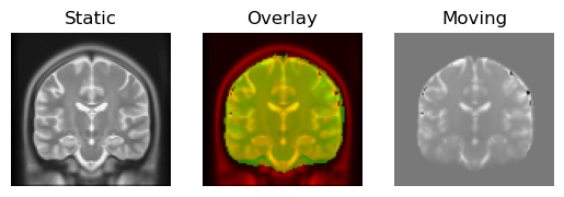
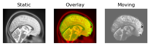
<Figure size 640x480 with 3 Axes>

Deformable registration result.

Let’s now fetch a set of streamlines from the Stanford HARDI dataset. Those streamlines were generated during the Connectivity Matrices, ROI Intersections and Density Maps example.

We read the streamlines from file in voxel space:

streamlines_files = fetch_stanford_tracks()
lr_superiorfrontal_path = pjoin(streamlines_files[1],
                                'hardi-lr-superiorfrontal.trk')

sft = load_tractogram(lr_superiorfrontal_path, 'same')

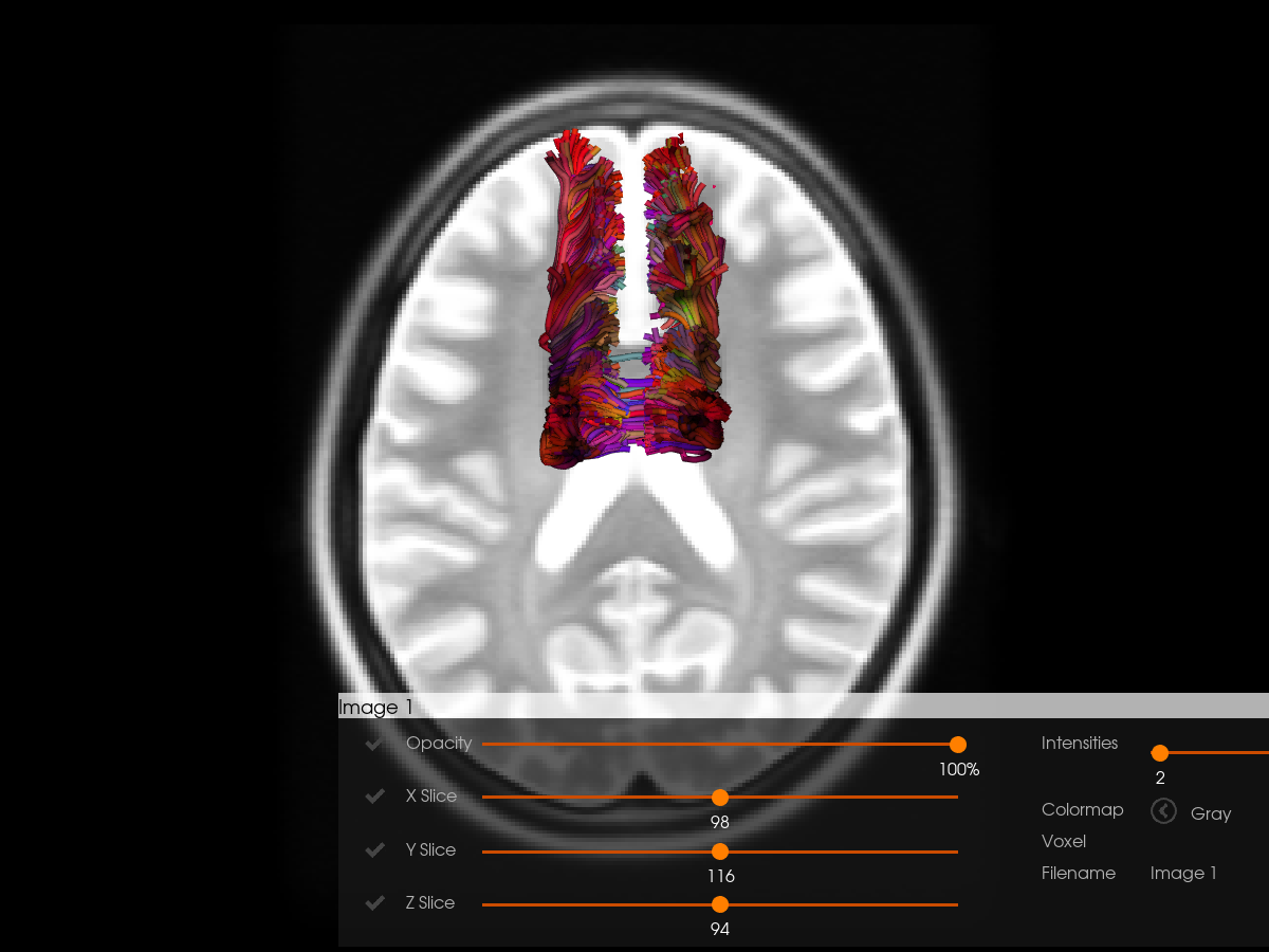
The affine registration already gives a pretty good result. We could use its mapping to transform the streamlines to the anatomical space (MNI T2 image). For that, we use transform_streamlines and warped_b0_affine. Do not forget that warp_b0_affine is the affine transformation from the mean b0 image to the T2 template image. Thus, you typically need to apply the inverse transformation of the affine transformation matrix that was used to register the two images. This is because the transformation matrix describes how points in one image (mean_b0) are mapped to points in the other image (mni T2), and to move points from the warped_b0 space to the t2 space, you need to “undo” this transformation.

mni_t2_streamlines_using_affine_reg = transform_streamlines(
        sft.streamlines, np.linalg.inv(warped_b0_affine))

sft_in_t2_using_aff_reg = StatefulTractogram(
      mni_t2_streamlines_using_affine_reg, img_t2_mni, Space.RASMM)

Let’s visualize the streamlines in the MNI T2 space. Switch the interactive variable to True if you want to explore the visualization in an interactive window.

interactive = False

if has_fury:
    horizon(tractograms=[sft_in_t2_using_aff_reg],
            images=[(t2_mni_data, t2_mni_affine)],
            interactive=interactive, world_coords=True,
            out_png='streamlines_DSN_MNI_aff_reg.png')

Original shape: (197, 233, 189)
Resized to RAS shape: (197, 233, 189)

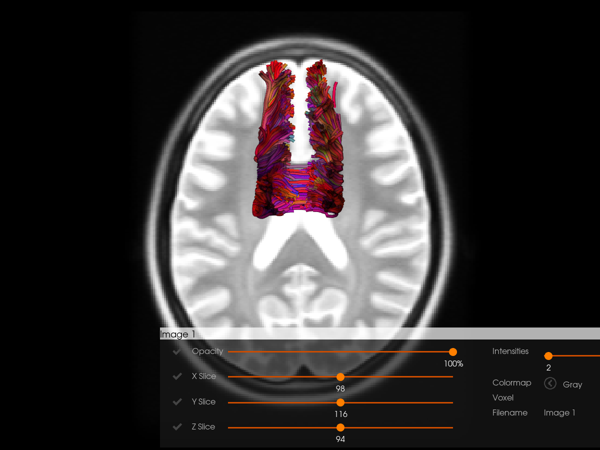
To get better result, we use the mapping obtain by Symmetric Diffeomorphic Registration (SyN). Then, we can visualize the corpus callosum bundles that have been deformed to adapt to the MNI template space.

mni_t2_streamlines_using_syn = mapping.transform_points_inverse(
    sft.streamlines)

sft_in_t2_using_syn = StatefulTractogram(
    mni_t2_streamlines_using_syn, img_t2_mni, Space.RASMM)

if has_fury:
    horizon(tractograms=[sft_in_t2_using_syn],
            images=[(t2_mni_data, t2_mni_affine)],
            interactive=interactive, world_coords=True,
            out_png='streamlines_DSN_MNI_syn.png')

Original shape: (197, 233, 189)
Resized to RAS shape: (197, 233, 189)

Finally, we save the two registered streamlines:

• mni-lr-sft_in_t2_using_aff_reg.trk is the streamlines registered using the affine registration.

• sft_in_t2_using_syn is the streamlines registered using the SyN registration and prealigned with the affine registration.

save_tractogram(sft_in_t2_using_aff_reg, 'mni-lr-superiorfrontal_aff_reg.trk',
                bbox_valid_check=False)

save_tractogram(sft_in_t2_using_syn, 'mni-lr-superiorfrontal_syn.trk',
                bbox_valid_check=False)

True

References

[Avants09]

Avants, B. B., Epstein, C. L., Grossman, M., & Gee, J. C. (2009). Symmetric Diffeomorphic Image Registration with Cross-Correlation: Evaluating Automated Labeling of Elderly and Neurodegenerative Brain, 12(1), 26-41.

[Avants11]

Avants, B. B., Tustison, N., & Song, G. (2011). Advanced Normalization Tools (ANTS), 1-35.

[Greene17]

Greene, C., Cieslak, M., & Grafton, S. T. (2017). Effect of different spatial normalization approaches on tractography and structural brain networks. Network Neuroscience, 1-19.