Reconstruction with Constrained Spherical Deconvolution model (CSD)

This example shows how to use Constrained Spherical Deconvolution (CSD) introduced by [1].

This method is mainly useful with datasets with gradient directions acquired on a spherical grid.

The basic idea with this method is that if we could estimate the response function of a single fiber then we could deconvolve the measured signal and obtain the underlying fiber distribution.

In this way, the reconstruction of the fiber orientation distribution function (fODF) in CSD involves two steps:

1. Estimation of the fiber response function

2. Use the response function to reconstruct the fODF

Let’s first load the data. We will use a dataset with 10 b0s and 150 non-b0s with b-value 2000.

import numpy as np

from dipy.core.gradients import gradient_table
from dipy.data import default_sphere, get_fnames
from dipy.direction import peaks_from_model
from dipy.io.gradients import read_bvals_bvecs
from dipy.io.image import load_nifti
from dipy.reconst.csdeconv import (
    ConstrainedSphericalDeconvModel,
    auto_response_ssst,
    mask_for_response_ssst,
    recursive_response,
    response_from_mask_ssst,
)
from dipy.reconst.dti import TensorModel, fractional_anisotropy, mean_diffusivity
from dipy.sims.voxel import single_tensor_odf
from dipy.viz import actor, window

hardi_fname, hardi_bval_fname, hardi_bvec_fname = get_fnames(name="stanford_hardi")

data, affine = load_nifti(hardi_fname)

bvals, bvecs = read_bvals_bvecs(hardi_bval_fname, hardi_bvec_fname)
gtab = gradient_table(bvals, bvecs=bvecs)

You can verify the b-values of the dataset by looking at the attribute gtab.bvals. Now that a dataset with multiple gradient directions is loaded, we can proceed with the two steps of CSD.

Step 1. Estimation of the fiber response function

There are many strategies to estimate the fiber response function. Here two different strategies are presented.

Strategy 1 - response function estimates from a local brain region One simple way to estimate the fiber response function is to look for regions of the brain where it is known that there are single coherent fiber populations. For example, if we use a ROI at the center of the brain, we will find single fibers from the corpus callosum. The auto_response_ssst function will calculate FA for a cuboid ROI of radii equal to roi_radii in the center of the volume and return the response function estimated in that region for the voxels with FA higher than 0.7.

response, ratio = auto_response_ssst(gtab, data, roi_radii=10, fa_thr=0.7)

Note that the auto_response_ssst function calls two functions that can be used separately. First, the function mask_for_response_ssst creates a mask of voxels within the cuboid ROI that meet the FA threshold constraint. This mask can be used to calculate the number of voxels that were kept, or to also apply an external mask (a WM mask for example). Second, the function response_from_mask_ssst takes the mask and returns the response function calculated within the mask. If no changes are made to the mask between the two calls, the resulting responses should be identical.

mask = mask_for_response_ssst(gtab, data, roi_radii=10, fa_thr=0.7)
nvoxels = np.sum(mask)
print(nvoxels)

response, ratio = response_from_mask_ssst(gtab, data, mask)

1254

The response tuple contains two elements. The first is an array with the eigenvalues of the response function and the second is the average S0 for this response.

It is good practice to always validate the result of auto_response_ssst. For this purpose we can print the elements of response and have a look at their values.

print(response)

(array([0.00139919, 0.0003007 , 0.0003007 ]), np.float64(416.7372408293461))

The tensor generated from the response must be prolate (two smaller eigenvalues should be equal) and look anisotropic with a ratio of second to first eigenvalue of about 0.2. Or in other words, the axial diffusivity of this tensor should be around 5 times larger than the radial diffusivity.

print(ratio)

0.21491283972216865

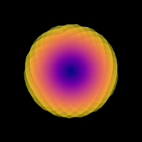
We can double-check that we have a good response function by visualizing the response function’s ODF. Here is how you would do that:

# Enables/disables interactive visualization
interactive = False

scene = window.Scene()
evals = response[0]
evecs = np.array([[0, 1, 0], [0, 0, 1], [1, 0, 0]]).T


response_odf = single_tensor_odf(default_sphere.vertices, evals=evals, evecs=evecs)
# transform our data from 1D to 4D
response_odf = response_odf[None, None, None, :]
response_actor = actor.odf_slicer(
    response_odf, sphere=default_sphere, colormap="plasma"
)
scene.add(response_actor)
print("Saving illustration as csd_response.png")
window.record(scene=scene, out_path="csd_response.png", size=(200, 200))
if interactive:
    window.show(scene)

Saving illustration as csd_response.png

Estimated response function.

scene.rm(response_actor)

Strategy 2 - data-driven calibration of response function Depending on the dataset, FA threshold may not be the best way to find the best possible response function. For one, it depends on the diffusion tensor (FA and first eigenvector), which has lower accuracy at high b-values. Alternatively, the response function can be calibrated in a data-driven manner [2].

First, the data is deconvolved with a ‘fat’ response function. All voxels that are considered to contain only one peak in this deconvolution (as determined by the peak threshold which gives an upper limit of the ratio of the second peak to the first peak) are maintained, and from these voxels a new response function is determined. This process is repeated until convergence is reached. Here we calibrate the response function on a small part of the data.

A WM mask can shorten computation time for the whole dataset. Here it is created based on the DTI fit.

tenmodel = TensorModel(gtab)
tenfit = tenmodel.fit(data, mask=data[..., 0] > 200)

FA = fractional_anisotropy(tenfit.evals)
MD = mean_diffusivity(tenfit.evals)
wm_mask = np.logical_or(FA >= 0.4, (np.logical_and(FA >= 0.15, MD >= 0.0011)))

response = recursive_response(
    gtab,
    data,
    mask=wm_mask,
    sh_order_max=8,
    peak_thr=0.01,
    init_fa=0.08,
    init_trace=0.0021,
    iter=8,
    convergence=0.001,
    parallel=True,
    num_processes=2,
)

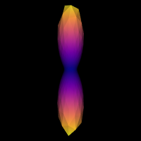
We can check the shape of the signal of the response function, which should be like a pancake:

response_signal = response.on_sphere(default_sphere)
# transform our data from 1D to 4D
response_signal = response_signal[None, None, None, :]
response_actor = actor.odf_slicer(
    response_signal, sphere=default_sphere, colormap="plasma"
)

scene = window.Scene()

scene.add(response_actor)
print("Saving illustration as csd_recursive_response.png")
window.record(scene=scene, out_path="csd_recursive_response.png", size=(200, 200))
if interactive:
    window.show(scene)

Saving illustration as csd_recursive_response.png

Estimated response function using recursive calibration.

scene.rm(response_actor)

Step 2. fODF reconstruction

After estimating a response function for one of the strategies shown above, we are ready to start the deconvolution process. Let’s import the CSD model and fit the datasets.

csd_model = ConstrainedSphericalDeconvModel(gtab, response)

For illustration purposes we will fit only a small portion of the data.

data_small = data[20:50, 55:85, 38:39]
csd_fit = csd_model.fit(data_small)

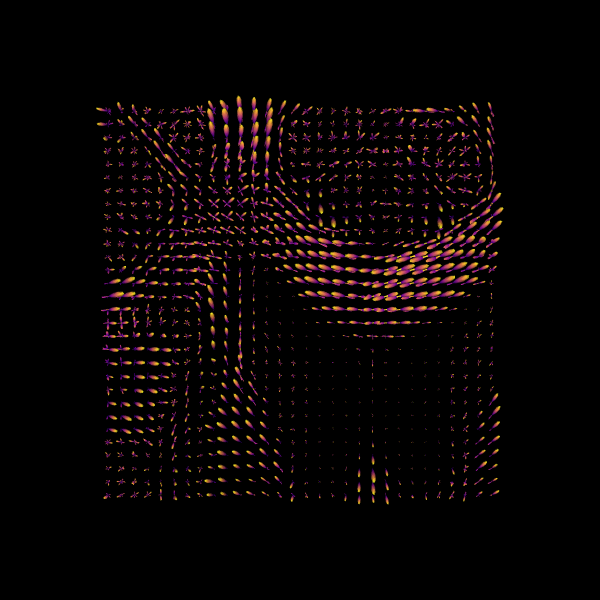
Show the CSD-based ODFs also known as FODFs (fiber ODFs).

csd_odf = csd_fit.odf(default_sphere)

Here we visualize only a 30x30 region.

fodf_spheres = actor.odf_slicer(
    csd_odf, sphere=default_sphere, scale=0.9, norm=False, colormap="plasma"
)

scene.add(fodf_spheres)

print("Saving illustration as csd_odfs.png")
window.record(scene=scene, out_path="csd_odfs.png", size=(600, 600))
if interactive:
    window.show(scene)

Saving illustration as csd_odfs.png

CSD ODFs.

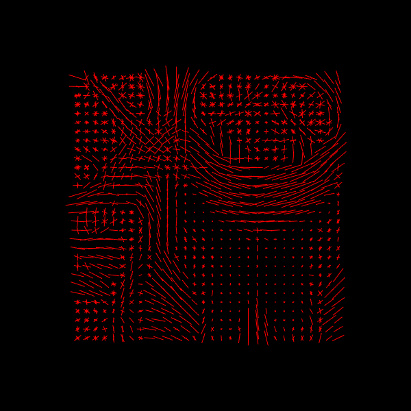
In DIPY we also provide tools for finding the peak directions (maxima) of the ODFs. For this purpose we recommend using peaks_from_model.

csd_peaks = peaks_from_model(
    model=csd_model,
    data=data_small,
    sphere=default_sphere,
    relative_peak_threshold=0.5,
    min_separation_angle=25,
    parallel=True,
    num_processes=2,
)

scene.clear()
fodf_peaks = actor.peak_slicer(csd_peaks.peak_dirs, peaks_values=csd_peaks.peak_values)
scene.add(fodf_peaks)

print("Saving illustration as csd_peaks.png")
window.record(scene=scene, out_path="csd_peaks.png", size=(600, 600))
if interactive:
    window.show(scene)

Saving illustration as csd_peaks.png

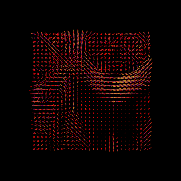
CSD Peaks.

We can finally visualize both the ODFs and peaks in the same space.

fodf_spheres.GetProperty().SetOpacity(0.4)

scene.add(fodf_spheres)

print("Saving illustration as csd_both.png")
window.record(scene=scene, out_path="csd_both.png", size=(600, 600))
if interactive:
    window.show(scene)

Saving illustration as csd_both.png

CSD Peaks and ODFs.

References

[1]

Jacques-Donald Tournier, Fernando Calamante, and Alan Connelly. Robust determination of the fibre orientation distribution in diffusion MRI: Non-negativity constrained super-resolved spherical deconvolution. NeuroImage, 35(4):1459–1472, May 2007. URL: https://doi.org/10.1016/j.neuroimage.2012.06.005, doi:10.1016/j.neuroimage.2007.02.016.

[2]

Chantal M.W. Tax, Ben Jeurissen, Sjoerd B. Vos, Max A. Viergever, and Alexander Leemans. Recursive calibration of the fiber response function for spherical deconvolution of diffusion MRI data. NeuroImage, 86:67–80, 2014. URL: https://doi.org/10.1016/j.neuroimage.2013.07.067, doi:10.1016/j.neuroimage.2013.07.067.