MultiTensor Simulation

In this example we show how someone can simulate the signal and the ODF of a single voxel using a MultiTensor.

import matplotlib.pyplot as plt
import numpy as np

from dipy.core.sphere import disperse_charges, HemiSphere
from dipy.core.gradients import gradient_table
from dipy.data import get_sphere
from dipy.sims.voxel import multi_tensor, multi_tensor_odf
from dipy.viz import window, actor

For the simulation we will need a GradientTable with the b-values and b-vectors. To create one, we can first create some random points on a HemiSphere using spherical polar coordinates.

rng = np.random.default_rng()

n_pts = 64
theta = np.pi * rng.random(size=n_pts)
phi = 2 * np.pi * rng.random(size=n_pts)
hsph_initial = HemiSphere(theta=theta, phi=phi)

Next, we call disperse_charges which will iteratively move the points so that the electrostatic potential energy is minimized.

hsph_updated, potential = disperse_charges(hsph_initial, 5000)

We need two stacks of vertices, one for every shell, and we need two sets of b-values, one at 1000 \(s/mm^2\), and one at 2500 \(s/mm^2\), as we discussed previously.

vertices = hsph_updated.vertices
values = np.ones(vertices.shape[0])

bvecs = np.vstack((vertices, vertices))
bvals = np.hstack((1000 * values, 2500 * values))

We can also add some b0s. Let’s add one at the beginning and one at the end.

bvecs = np.insert(bvecs, (0, bvecs.shape[0]), np.array([0, 0, 0]), axis=0)
bvals = np.insert(bvals, (0, bvals.shape[0]), 0)

Let’s now create the GradientTable.

gtab = gradient_table(bvals, bvecs)

In mevals we save the eigenvalues of each tensor.

mevals = np.array([[0.0015, 0.0003, 0.0003],
                   [0.0015, 0.0003, 0.0003]])

In angles we save in polar coordinates (\(\theta, \phi\)) the principal axis of each tensor.

angles = [(0, 0), (60, 0)]

In fractions we save the percentage of the contribution of each tensor.

fractions = [50, 50]

The function multi_tensor will return the simulated signal and an array with the principal axes of the tensors in cartesian coordinates.

signal, sticks = multi_tensor(gtab, mevals, S0=100, angles=angles,
                              fractions=fractions, snr=None)

We can also add Rician noise with a specific SNR.

signal_noisy, sticks = multi_tensor(gtab, mevals, S0=100, angles=angles,
                                    fractions=fractions, snr=20)

plt.plot(signal, label='noiseless')

plt.plot(signal_noisy, label='with noise')
plt.legend()
# plt.show()
plt.savefig('simulated_signal.png', bbox_inches='tight')

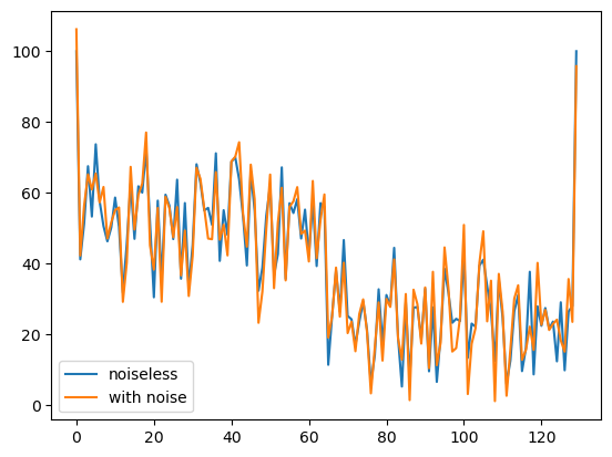
Simulated MultiTensor signal

For the ODF simulation we will need a sphere. Because we are interested in a simulation of only a single voxel, we can use a sphere with very high resolution. We generate that by subdividing the triangles of one of DIPY’s cached spheres, which we can read in the following way.

sphere = get_sphere('repulsion724')
sphere = sphere.subdivide(2)

odf = multi_tensor_odf(sphere.vertices, mevals, angles, fractions)

# Enables/disables interactive visualization
interactive = False

scene = window.Scene()

odf_actor = actor.odf_slicer(odf[None, None, None, :], sphere=sphere,
                             colormap='plasma')
odf_actor.RotateX(90)

scene.add(odf_actor)

print('Saving illustration as multi_tensor_simulation')
window.record(scene, out_path='multi_tensor_simulation.png', size=(300, 300))
if interactive:
    window.show(scene)

Saving illustration as multi_tensor_simulation

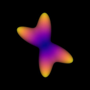
Simulating a MultiTensor ODF.