Calculate Path Length Map

We show how to calculate a Path Length Map for Anisotropic Radiation Therapy Contours given a set of streamlines and a region of interest (ROI). The Path Length Map is a volume in which each voxel’s value is the shortest distance along a streamline to a given region of interest (ROI). This map can be used to anisotropically modify radiation therapy treatment contours based on a tractography model of the local white matter anatomy, as described in [Jordan_2018_plm], by executing this tutorial with the gross tumor volume (GTV) as the ROI.

Note

The background value is set to -1 by default

Let’s start by importing the necessary modules.

from dipy.core.gradients import gradient_table
from dipy.data import get_fnames, default_sphere
from dipy.io.gradients import read_bvals_bvecs
from dipy.io.image import load_nifti_data, load_nifti, save_nifti
from dipy.reconst.shm import CsaOdfModel
from dipy.direction import peaks_from_model
from dipy.tracking.stopping_criterion import ThresholdStoppingCriterion
from dipy.tracking import utils
from dipy.tracking.local_tracking import LocalTracking
from dipy.tracking.streamline import Streamlines
from dipy.viz import actor, window, colormap as cmap
from dipy.tracking.utils import path_length
import numpy as np
import matplotlib as mpl
from mpl_toolkits.axes_grid1 import AxesGrid

First, we need to generate some streamlines and visualize. For a more complete description of these steps, please refer to the An introduction to the Probabilistic Direction Getter and the Visualization of ROI Surface Rendered with Streamlines Tutorials.

hardi_fname, hardi_bval_fname, hardi_bvec_fname = get_fnames('stanford_hardi')
label_fname = get_fnames('stanford_labels')

data, affine, hardi_img = load_nifti(hardi_fname, return_img=True)
labels = load_nifti_data(label_fname)

bvals, bvecs = read_bvals_bvecs(hardi_bval_fname, hardi_bvec_fname)
gtab = gradient_table(bvals, bvecs)

white_matter = (labels == 1) | (labels == 2)

csa_model = CsaOdfModel(gtab, sh_order_max=6)
csa_peaks = peaks_from_model(csa_model, data, default_sphere,
                             relative_peak_threshold=.8,
                             min_separation_angle=45,
                             mask=white_matter)

stopping_criterion = ThresholdStoppingCriterion(csa_peaks.gfa, .25)

We will use an anatomically-based corpus callosum ROI as our seed mask to demonstrate the method. In practice, this corpus callosum mask (labels == 2) should be replaced with the desired ROI mask (e.g. gross tumor volume (GTV), lesion mask, or electrode mask).

# Make a corpus callosum seed mask for tracking
seed_mask = labels == 2
seeds = utils.seeds_from_mask(seed_mask, affine, density=[1, 1, 1])

# Make a streamline bundle model of the corpus callosum ROI connectivity
streamlines = LocalTracking(csa_peaks, stopping_criterion, seeds, affine,
                            step_size=2)
streamlines = Streamlines(streamlines)

# Visualize the streamlines and the Path Length Map base ROI
# (in this case also the seed ROI)

streamlines_actor = actor.line(streamlines, cmap.line_colors(streamlines))
surface_opacity = 0.5
surface_color = [0, 1, 1]
seedroi_actor = actor.contour_from_roi(seed_mask, affine,
                                       surface_color, surface_opacity)

scene = window.Scene()
scene.add(streamlines_actor)
scene.add(seedroi_actor)

If you set interactive to True (below), the scene will pop up in an interactive window.

interactive = False
if interactive:
    window.show(scene)

window.record(scene, n_frames=1, out_path='plm_roi_sls.png',
              size=(800, 800))

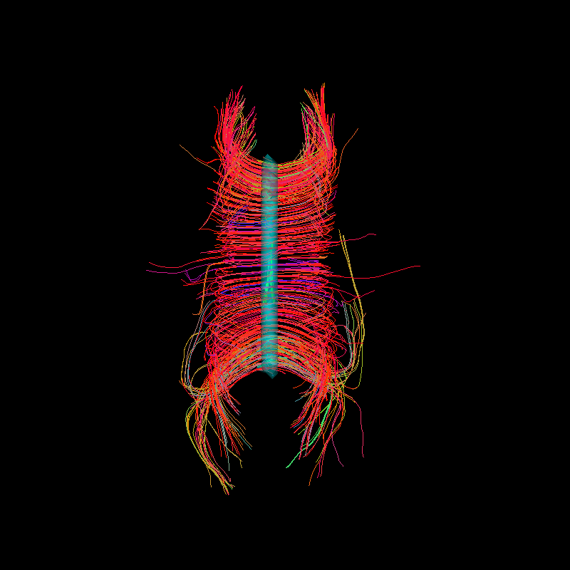
A top view of corpus callosum streamlines with the blue transparent ROI in the center.

Now we calculate the Path Length Map using the corpus callosum streamline bundle and corpus callosum ROI.

NOTE: the mask used to seed the tracking does not have to be the Path Length Map base ROI, as we do here, but it often makes sense for them to be the same ROI if we want a map of the whole brain’s distance back to our ROI. (e.g. we could test a hypothesis about the motor system by making a streamline bundle model of the cortico-spinal track (CST) and input a lesion mask as our Path Length Map base ROI to restrict the analysis to the CST)

path_length_map_base_roi = seed_mask

# calculate the WMPL
wmpl = path_length(streamlines, affine, path_length_map_base_roi)

# save the WMPL as a nifti
save_nifti('example_cc_path_length_map.nii.gz', wmpl.astype(np.float32),
           affine)

# get the T1 to show anatomical context of the WMPL
t1_fname = get_fnames('stanford_t1')
t1_data = load_nifti_data(t1_fname)


fig = mpl.pyplot.figure()
fig.subplots_adjust(left=0.05, right=0.95)
ax = AxesGrid(fig, 111,
              nrows_ncols=(1, 3),
              cbar_location="right",
              cbar_mode="single",
              cbar_size="10%",
              cbar_pad="5%")

We will mask our WMPL to ignore values less than zero because negative numbers indicate no path back to the ROI was found in the provided streamlines

wmpl_show = np.ma.masked_where(wmpl < 0, wmpl)

slx, sly, slz = [60, 50, 35]
ax[0].matshow(np.rot90(t1_data[:, slx, :]), cmap=mpl.cm.bone)
im = ax[0].matshow(np.rot90(wmpl_show[:, slx, :]),
                   cmap=mpl.cm.cool, vmin=0, vmax=80)

ax[1].matshow(np.rot90(t1_data[:, sly, :]), cmap=mpl.cm.bone)
im = ax[1].matshow(np.rot90(wmpl_show[:, sly, :]), cmap=mpl.cm.cool,
                   vmin=0, vmax=80)

ax[2].matshow(np.rot90(t1_data[:, slz, :]), cmap=mpl.cm.bone)
im = ax[2].matshow(np.rot90(wmpl_show[:, slz, :]),
                   cmap=mpl.cm.cool, vmin=0, vmax=80)

ax.cbar_axes[0].colorbar(im)
for lax in ax:
    lax.set_xticks([])
    lax.set_yticks([])
fig.savefig("Path_Length_Map.png")

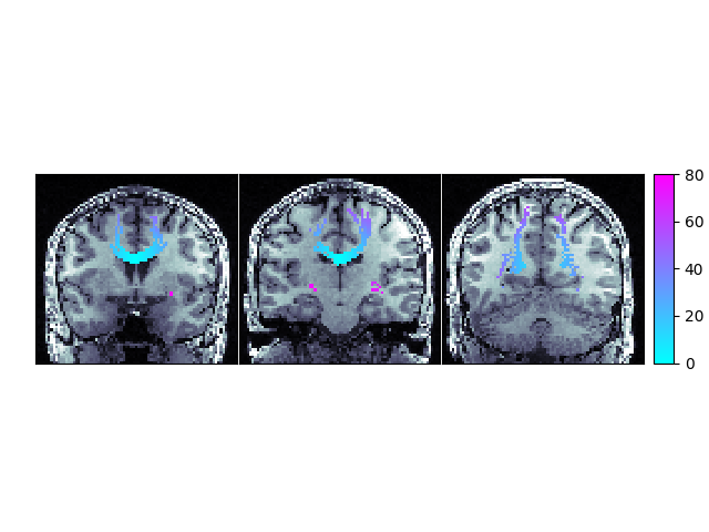
Path Length Map showing the shortest distance, along a streamline, from the corpus callosum ROI with the background set to -1.

References

[Jordan_2018_plm]

Jordan K. et al., “An Open-Source Tool for Anisotropic

Radiation Therapy Planning in Neuro-oncology Using DW-MRI Tractography”, PREPRINT (biorxiv), 2018.