Note
Go to the end to download the full example code.
Affine Registration in 3D#
This example explains how to compute an affine transformation to register two 3D volumes by maximization of their Mutual Information [1]. The optimization strategy is similar to that implemented in ANTS [2].
We will do this twice. The first part of this tutorial will walk through the
details of the process with the object-oriented interface implemented in
the dipy.align module. The second part will use a simplified functional
interface.
from pathlib import Path

import numpy as np

from dipy.align import affine_registration, register_dwi_to_template
from dipy.align.imaffine import (
    AffineMap,
    AffineRegistration,
    MutualInformationMetric,
    transform_centers_of_mass,
)
from dipy.align.transforms import (
    AffineTransform3D,
    RigidTransform3D,
    TranslationTransform3D,
)
from dipy.data import fetch_stanford_hardi
from dipy.data.fetcher import fetch_syn_data
from dipy.io.image import load_nifti
from dipy.viz import regtools
Let’s fetch two b0 volumes, the static image will be the b0 from the Stanford HARDI dataset
files, folder = fetch_stanford_hardi()
static_data, static_affine, static_img = load_nifti(
    Path(folder) / "HARDI150.nii.gz", return_img=True
)
static = np.squeeze(static_data)[..., 0]
static_grid2world = static_affine
Now the moving image
files, folder2 = fetch_syn_data()
moving_data, moving_affine, moving_img = load_nifti(
    Path(folder2) / "b0.nii.gz", return_img=True
)
moving = moving_data
moving_grid2world = moving_affine
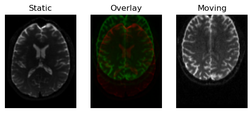
We can see that the images are far from aligned by drawing one on top of the other. The images don’t even have the same number of voxels, so in order to draw one on top of the other we need to resample the moving image on a grid of the same dimensions as the static image, we can do this by “transforming” the moving image using an identity transform
identity = np.eye(4)
affine_map = AffineMap(
    identity,
    domain_grid_shape=static.shape,
    domain_grid2world=static_grid2world,
    codomain_grid_shape=moving.shape,
    codomain_grid2world=moving_grid2world,
)
resampled = affine_map.transform(moving)
regtools.overlay_slices(
    static,
    resampled,
    slice_index=None,
    slice_type=0,
    ltitle="Static",
    rtitle="Moving",
    fname="resampled_0.png",
)
regtools.overlay_slices(
    static,
    resampled,
    slice_index=None,
    slice_type=1,
    ltitle="Static",
    rtitle="Moving",
    fname="resampled_1.png",
)
regtools.overlay_slices(
    static,
    resampled,
    slice_index=None,
    slice_type=2,
    ltitle="Static",
    rtitle="Moving",
    fname="resampled_2.png",
)
<Figure size 640x480 with 3 Axes>
Input images before alignment.
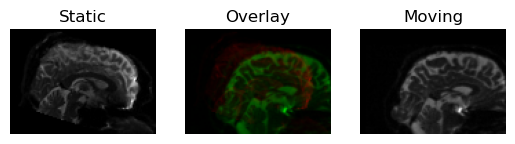
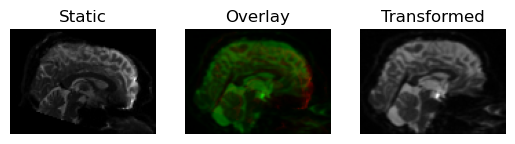
We can obtain a very rough (and fast) registration by just aligning the centers of mass of the two images
c_of_mass = transform_centers_of_mass(
    static,
    static_grid2world,
    moving,
    moving_grid2world,
)
We can now transform the moving image and draw it on top of the static image, registration is not likely to be good, but at least they will occupy roughly the same space
transformed = c_of_mass.transform(moving)
regtools.overlay_slices(
    static,
    transformed,
    slice_index=None,
    slice_type=0,
    ltitle="Static",
    rtitle="Transformed",
    fname="transformed_com_0.png",
)
regtools.overlay_slices(
    static,
    transformed,
    slice_index=None,
    slice_type=1,
    ltitle="Static",
    rtitle="Transformed",
    fname="transformed_com_1.png",
)
regtools.overlay_slices(
    static,
    transformed,
    slice_index=None,
    slice_type=2,
    ltitle="Static",
    rtitle="Transformed",
    fname="transformed_com_2.png",
)

<Figure size 640x480 with 3 Axes>
Registration result by aligning the centers of mass of the images.
This was just a translation of the moving image towards the static image, now we will refine it by looking for an affine transform. We first create the similarity metric (Mutual Information) to be used. We need to specify the number of bins to be used to discretize the joint and marginal probability distribution functions (PDF), a typical value is 32. We also need to specify the percentage (an integer in (0, 100]) of voxels to be used for computing the PDFs, the most accurate registration will be obtained by using all voxels, but it is also the most time-consuming choice. We specify full sampling by passing None instead of an integer
nbins = 32
sampling_prop = None
metric = MutualInformationMetric(nbins=nbins, sampling_proportion=sampling_prop)
To avoid getting stuck at local optima, and to accelerate convergence, we use a multi-resolution strategy (similar to ANTS [2]) by building a Gaussian Pyramid. To have as much flexibility as possible, the user can specify how this Gaussian Pyramid is built. First of all, we need to specify how many resolutions we want to use. This is indirectly specified by just providing a list of the number of iterations we want to perform at each resolution. Here we will just specify 3 resolutions and a large number of iterations, 10000 at the coarsest resolution, 1000 at the medium resolution and 100 at the finest. These are the default settings
level_iters = [10000, 1000, 100]
To compute the Gaussian pyramid, the original image is first smoothed at each level of the pyramid using a Gaussian kernel with the requested sigma. A good initial choice is [3.0, 1.0, 0.0], this is the default
sigmas = [3.0, 1.0, 0.0]
Now we specify the sub-sampling factors. A good configuration is [4, 2, 1], which means that, if the original image shape was (nx, ny, nz) voxels, then the shape of the coarsest image will be about (nx//4, ny//4, nz//4), the shape in the middle resolution will be about (nx//2, ny//2, nz//2) and the image at the finest scale has the same size as the original image. This set of factors is the default
factors = [4, 2, 1]
Now we go ahead and instantiate the registration class with the configuration we just prepared
Using AffineRegistration we can register our images in as many stages as we want, providing previous results as initialization for the next (the same logic as in ANTS). The reason why it is useful is that registration is a non-convex optimization problem (it may have more than one local optima), which means that it is very important to initialize as close to the solution as possible. For example, let’s start with our (previously computed) rough transformation aligning the centers of mass of our images, and then refine it in three stages. First look for an optimal translation. The dictionary regtransforms contains all available transforms, we obtain one of them by providing its name and the dimension (either 2 or 3) of the image we are working with (since we are aligning volumes, the dimension is 3)
transform = TranslationTransform3D()
params0 = None
starting_affine = c_of_mass.affine
translation = affreg.optimize(
    static,
    moving,
    transform,
    params0,
    static_grid2world=static_grid2world,
    moving_grid2world=moving_grid2world,
    starting_affine=starting_affine,
)
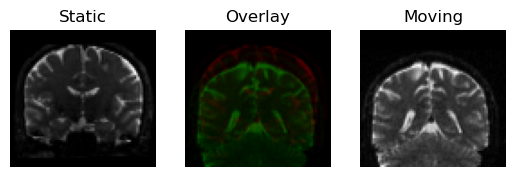
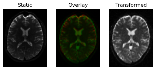
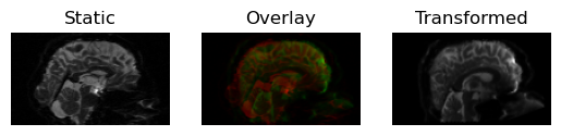
If we look at the result, we can see that this translation is much better than simply aligning the centers of mass
transformed = translation.transform(moving)
regtools.overlay_slices(
    static,
    transformed,
    slice_index=None,
    slice_type=0,
    ltitle="Static",
    rtitle="Transformed",
    fname="transformed_trans_0.png",
)
regtools.overlay_slices(
    static,
    transformed,
    slice_index=None,
    slice_type=1,
    ltitle="Static",
    rtitle="Transformed",
    fname="transformed_trans_1.png",
)
regtools.overlay_slices(
    static,
    transformed,
    slice_index=None,
    slice_type=2,
    ltitle="Static",
    rtitle="Transformed",
    fname="transformed_trans_2.png",
)

<Figure size 640x480 with 3 Axes>
Registration result by translating the moving image, using Mutual Information.
Now let’s refine with a rigid transform (this may even modify our previously found optimal translation)
transform = RigidTransform3D()
params0 = None
starting_affine = translation.affine
rigid = affreg.optimize(
    static,
    moving,
    transform,
    params0,
    static_grid2world=static_grid2world,
    moving_grid2world=moving_grid2world,
    starting_affine=starting_affine,
)
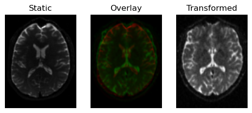
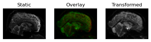
This produces a slight rotation, and the images are now better aligned
transformed = rigid.transform(moving)
regtools.overlay_slices(
    static,
    transformed,
    slice_index=None,
    slice_type=0,
    ltitle="Static",
    rtitle="Transformed",
    fname="transformed_rigid_0.png",
)
regtools.overlay_slices(
    static,
    transformed,
    slice_index=None,
    slice_type=1,
    ltitle="Static",
    rtitle="Transformed",
    fname="transformed_rigid_1.png",
)
regtools.overlay_slices(
    static,
    transformed,
    slice_index=None,
    slice_type=2,
    ltitle="Static",
    rtitle="Transformed",
    fname="transformed_rigid_2.png",
)
<Figure size 640x480 with 3 Axes>
Registration result with a rigid transform, using Mutual Information.
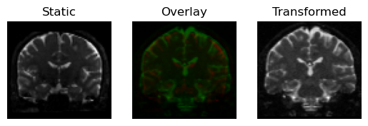
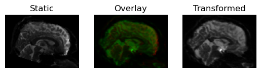
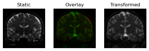
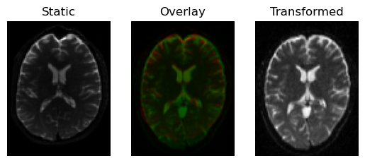
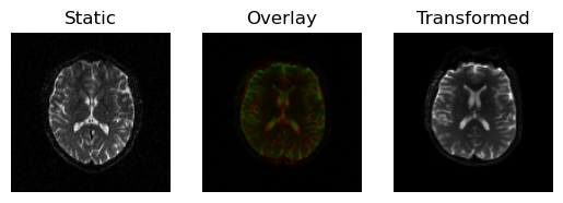
Finally, let’s refine with a full affine transform (translation, rotation, scale and shear), it is safer to fit more degrees of freedom now since we must be very close to the optimal transform
transform = AffineTransform3D()
params0 = None
starting_affine = rigid.affine
affine = affreg.optimize(
    static,
    moving,
    transform,
    params0,
    static_grid2world=static_grid2world,
    moving_grid2world=moving_grid2world,
    starting_affine=starting_affine,
)
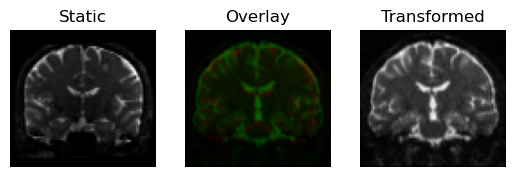
This results in a slight shear and scale
transformed = affine.transform(moving)
regtools.overlay_slices(
    static,
    transformed,
    slice_index=None,
    slice_type=0,
    ltitle="Static",
    rtitle="Transformed",
    fname="transformed_affine_0.png",
)
regtools.overlay_slices(
    static,
    transformed,
    slice_index=None,
    slice_type=1,
    ltitle="Static",
    rtitle="Transformed",
    fname="transformed_affine_1.png",
)
regtools.overlay_slices(
    static,
    transformed,
    slice_index=None,
    slice_type=2,
    ltitle="Static",
    rtitle="Transformed",
    fname="transformed_affine_2.png",
)


<Figure size 640x480 with 3 Axes>
Registration result with an affine transform, using Mutual Information.
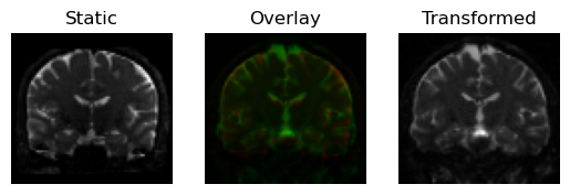
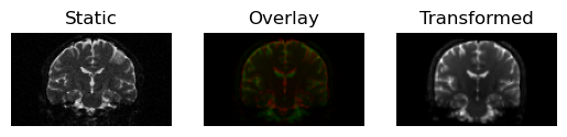
Now, let’s repeat this process with a simplified functional interface. This interface constructs a pipeline of operations from a given list of transformations.
pipeline = ["center_of_mass", "translation", "rigid", "affine"]
And then applies the transformations in the pipeline on the input (from left to right) with a call to an affine_registration function, which takes optional settings for things like the iterations, sigmas and factors. The pipeline must be a list of strings with one or more of the following transformations: center_of_mass, translation, rigid, rigid_isoscaling, rigid_scaling and affine.
xformed_img, reg_affine = affine_registration(
    moving,
    static,
    moving_affine=moving_affine,
    static_affine=static_affine,
    nbins=32,
    metric="MI",
    pipeline=pipeline,
    level_iters=level_iters,
    sigmas=sigmas,
    factors=factors,
)

regtools.overlay_slices(
    static,
    xformed_img,
    slice_index=None,
    slice_type=0,
    ltitle="Static",
    rtitle="Transformed",
    fname="xformed_affine_0.png",
)
regtools.overlay_slices(
    static,
    xformed_img,
    slice_index=None,
    slice_type=1,
    ltitle="Static",
    rtitle="Transformed",
    fname="xformed_affine_1.png",
)
regtools.overlay_slices(
    static,
    xformed_img,
    slice_index=None,
    slice_type=2,
    ltitle="Static",
    rtitle="Transformed",
    fname="xformed_affine_2.png",
)

<Figure size 640x480 with 3 Axes>
Registration result with an affine transform, using functional interface.
Alternatively, you can also use the register_dwi_to_template function that needs to also know about the gradient table of the DWI data, provided as a tuple of (bvals_file, bvecs_file). In this case, we are going to move the diffusion data to the B0 image (the opposite of the previous examples), which reverses what is the “moving” image and what is “static”.
xformed_dwi, reg_affine = register_dwi_to_template(
    dwi=static_img,
    gtab=(Path(folder) / "HARDI150.bval", Path(folder) / "HARDI150.bvec"),
    template=moving_img,
    reg_method="aff",
    nbins=32,
    metric="MI",
    pipeline=pipeline,
    level_iters=level_iters,
    sigmas=sigmas,
    factors=factors,
)

regtools.overlay_slices(
    moving,
    xformed_dwi,
    slice_index=None,
    slice_type=0,
    ltitle="Static",
    rtitle="Transformed",
    fname="xformed_dwi_0.png",
)
regtools.overlay_slices(
    moving,
    xformed_dwi,
    slice_index=None,
    slice_type=1,
    ltitle="Static",
    rtitle="Transformed",
    fname="xformed_dwi_1.png",
)
regtools.overlay_slices(
    moving,
    xformed_dwi,
    slice_index=None,
    slice_type=2,
    ltitle="Static",
    rtitle="Transformed",
    fname="xformed_dwi_2.png",
)
<Figure size 640x480 with 3 Axes>
Same again, using the dwi_to_template functional interface.
References#
Total running time of the script: (0 minutes 19.563 seconds)