Symmetric Diffeomorphic Registration in 2D

This example explains how to register 2D images using the Symmetric Normalization (SyN) algorithm proposed by Avants et al. [Avants09] (also implemented in the ANTs software [Avants11])

We will perform the classic Circle-To-C experiment for diffeomorphic registration

import numpy as np
from dipy.align.imwarp import SymmetricDiffeomorphicRegistration
from dipy.align.metrics import SSDMetric, CCMetric
import dipy.align.imwarp as imwarp
from dipy.data import get_fnames
from dipy.io.image import load_nifti_data
from dipy.segment.mask import median_otsu
from dipy.viz import regtools


fname_moving = get_fnames('reg_o')
fname_static = get_fnames('reg_c')

moving = np.load(fname_moving)
static = np.load(fname_static)

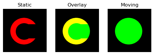
To visually check the overlap of the static image with the transformed moving image, we can plot them on top of each other with different channels to see where the differences are located

regtools.overlay_images(static, moving, 'Static', 'Overlay', 'Moving',
                        'input_images.png')

<Figure size 640x480 with 3 Axes>

Input images.

We want to find an invertible map that transforms the moving image (circle) into the static image (the C letter).

The first decision we need to make is what similarity metric is appropriate for our problem. In this example we are using two binary images, so the Sum of Squared Differences (SSD) is a good choice.

dim = static.ndim
metric = SSDMetric(dim)

Now we define an instance of the registration class. The SyN algorithm uses a multi-resolution approach by building a Gaussian Pyramid. We instruct the registration instance to perform at most \([n_0, n_1, ..., n_k]\) iterations at each level of the pyramid. The 0-th level corresponds to the finest resolution.

level_iters = [200, 100, 50, 25]

sdr = SymmetricDiffeomorphicRegistration(metric, level_iters, inv_iter=50)

Now we execute the optimization, which returns a DiffeomorphicMap object, that can be used to register images back and forth between the static and moving domains

mapping = sdr.optimize(static, moving)

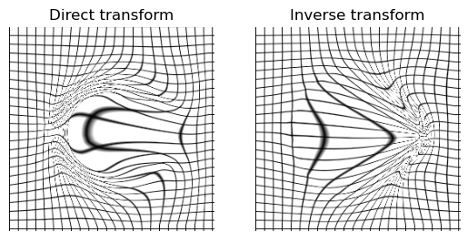
It is a good idea to visualize the resulting deformation map to make sure the result is reasonable (at least, visually)

regtools.plot_2d_diffeomorphic_map(mapping, 10, 'diffeomorphic_map.png')

(array([[  0.     ,   0.     ,   0.     , ...,   0.     ,   0.     ,
          0.     ],
       [  0.     , 127.     , 127.     , ...,   0.     , 127.     ,
        127.     ],
       [  0.     , 127.     , 126.99999, ...,   0.     , 127.     ,
        127.     ],
       ...,
       [  0.     ,   0.     ,   0.     , ...,   0.     ,   0.     ,
          0.     ],
       [  0.     , 127.     , 127.     , ...,   0.     , 127.     ,
        127.     ],
       [  0.     , 127.     , 127.     , ...,   0.     , 127.     ,
        127.     ]], dtype=float32), array([[  0.     ,   0.     ,   0.     , ...,   0.     ,   0.     ,
          0.     ],
       [  0.     , 126.88535, 126.92105, ...,   0.     , 127.     ,
        127.     ],
       [  0.     , 126.85171, 127.     , ...,   0.     , 127.     ,
        127.     ],
       ...,
       [  0.     ,   0.     ,   0.     , ...,   0.     ,   0.     ,
          0.     ],
       [  0.     , 127.     , 127.     , ...,   0.     , 127.     ,
        127.     ],
       [  0.     , 127.     , 127.     , ...,   0.     , 127.     ,
        127.     ]], dtype=float32))

Deformed lattice under the resulting diffeomorphic map.

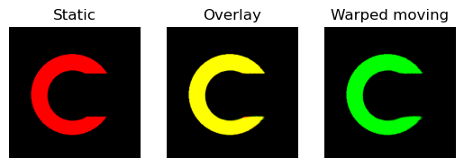
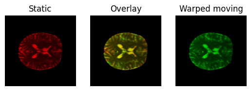
Now let’s warp the moving image and see if it gets similar to the static image

warped_moving = mapping.transform(moving, 'linear')
regtools.overlay_images(static, warped_moving, 'Static', 'Overlay',
                        'Warped moving', 'direct_warp_result.png')

<Figure size 640x480 with 3 Axes>

Moving image transformed under the (direct) transformation in green on top of the static image (in red).

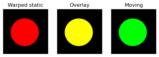
And we can also apply the inverse mapping to verify that the warped static image is similar to the moving image

warped_static = mapping.transform_inverse(static, 'linear')
regtools.overlay_images(warped_static, moving, 'Warped static', 'Overlay',
                        'Moving', 'inverse_warp_result.png')

<Figure size 640x480 with 3 Axes>

Static image transformed under the (inverse) transformation in red on top of the moving image (in green).

Now let’s register a couple of slices from a b0 image using the Cross Correlation metric. Also, let’s inspect the evolution of the registration. To do this we will define a function that will be called by the registration object at each stage of the optimization process. We will draw the current warped images after finishing each resolution.

def callback_CC(sdr, status):
    # Status indicates at which stage of the optimization we currently are
    # For now, we will only react at the end of each resolution of the scale
    # space
    if status == imwarp.RegistrationStages.SCALE_END:
        # get the current images from the metric
        wmoving = sdr.metric.moving_image
        wstatic = sdr.metric.static_image
        # draw the images on top of each other with different colors
        regtools.overlay_images(wmoving, wstatic, 'Warped moving', 'Overlay',
                                'Warped static')

Now we are ready to configure and run the registration. First load the data

t1_name, b0_name = get_fnames('syn_data')
data = load_nifti_data(b0_name)

We first remove the skull from the b0 volume

b0_mask, mask = median_otsu(data, median_radius=4, numpass=4)

And select two slices to try the 2D registration

static = b0_mask[:, :, 40]
moving = b0_mask[:, :, 38]

After loading the data, we instantiate the Cross-Correlation metric. The metric receives three parameters: the dimension of the input images, the standard deviation of the Gaussian Kernel to be used to regularize the gradient and the radius of the window to be used for evaluating the local normalized cross correlation.

sigma_diff = 3.0
radius = 4
metric = CCMetric(2, sigma_diff, radius)

Let’s use a scale space of 3 levels

level_iters = [100, 50, 25]
sdr = SymmetricDiffeomorphicRegistration(metric, level_iters)
sdr.callback = callback_CC

And execute the optimization

mapping = sdr.optimize(static, moving)

warped = mapping.transform(moving)

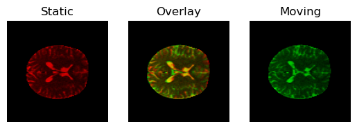
We can see the effect of the warping by switching between the images before and after registration

regtools.overlay_images(static, moving, 'Static', 'Overlay', 'Moving',
                        't1_slices_input.png')

<Figure size 640x480 with 3 Axes>

Input images.

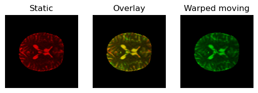
regtools.overlay_images(static, warped, 'Static', 'Overlay', 'Warped moving',
                        't1_slices_res.png')

<Figure size 640x480 with 3 Axes>

Moving image transformed under the (direct) transformation in green on top of the static image (in red).

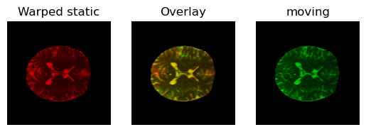
And we can apply the inverse warping too

inv_warped = mapping.transform_inverse(static)
regtools.overlay_images(inv_warped, moving, 'Warped static', 'Overlay',
                        'moving', 't1_slices_res2.png')

<Figure size 640x480 with 3 Axes>

Static image transformed under the (inverse) transformation in red on top of the moving image (in green).

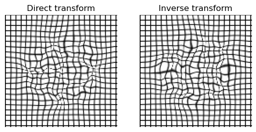
Finally, let’s see the deformation

regtools.plot_2d_diffeomorphic_map(mapping, 5, 'diffeomorphic_map_b0s.png')

(array([[  0.     ,   0.     ,   0.     , ...,   0.     ,   0.     ,
          0.     ],
       [  0.     , 126.99999, 127.00001, ..., 127.     ,   0.     ,
        127.     ],
       [  0.     , 127.     , 127.     , ..., 127.     ,   0.     ,
        127.     ],
       ...,
       [  0.     , 127.     , 127.     , ..., 127.     ,   0.     ,
        127.     ],
       [  0.     ,   0.     ,   0.     , ...,   0.     ,   0.     ,
          0.     ],
       [  0.     , 127.     , 127.     , ..., 127.     ,   0.     ,
        127.     ]], dtype=float32), array([[  0.      ,   0.      ,   0.      , ...,   0.      ,   0.      ,
          0.      ],
       [  0.      , 126.99708 , 126.999725, ..., 127.      ,   0.      ,
        127.      ],
       [  0.      , 126.99444 , 127.      , ..., 127.      ,   0.      ,
        127.      ],
       ...,
       [  0.      , 127.      , 127.      , ..., 127.      ,   0.      ,
        127.      ],
       [  0.      ,   0.      ,   0.      , ...,   0.      ,   0.      ,
          0.      ],
       [  0.      , 127.      , 127.      , ..., 127.      ,   0.      ,
        127.      ]], dtype=float32))

Deformed lattice under the resulting diffeomorphic map.

References

[Avants09]

Avants, B. B., Epstein, C. L., Grossman, M., & Gee, J. C. (2009). Symmetric Diffeomorphic Image Registration with Cross-Correlation: Evaluating Automated Labeling of Elderly and Neurodegenerative Brain, 12(1), 26-41.

[Avants11]

Avants, B. B., Tustison, N., & Song, G. (2011). Advanced Normalization Tools (ANTS), 1-35.