Continuous and analytical diffusion signal modelling with MAP-MRI

We show how to model the diffusion signal as a linear combination of continuous functions from the MAP-MRI basis [1]. This continuous representation allows for the computation of many properties of both the signal and diffusion propagator.

We show how to estimate the analytical orientation distribution function (ODF) and a variety of scalar indices. These include rotationally invariant quantities such as the mean squared displacement (MSD), Q-space inverse variance (QIV), teturn-to-origin probability (RTOP) and non-Gaussianity (NG). Interestingly, the MAP-MRI basis also allows for the computation of directional indices, such as the return-to-axis probability (RTAP), the return-to-plane probability (RTPP), and the parallel and perpendicular non-Gaussianity.

The estimation of these properties from noisy and sparse DWIs requires that the fitting of the MAP-MRI basis is constrained and/or regularized. This can be done by constraining the diffusion propagator to positive values [1], [2], and through analytic Laplacian regularization (MAPL) [3].

First import the necessary modules:

from dipy.core.gradients import gradient_table
from dipy.data import get_fnames, get_sphere
from dipy.io.gradients import read_bvals_bvecs
from dipy.io.image import load_nifti
from dipy.reconst import mapmri
from dipy.viz import actor, window
from dipy.viz.plotting import compare_maps

Download and read the data for this tutorial.

MAP-MRI requires multi-shell data, to properly fit the radial part of the basis. The total size of the downloaded data is 187.66 MBytes, however you only need to fetch it once.

fraw, fbval, fbvec, t1_fname = get_fnames(name="cfin_multib")

data contains the voxel data and gtab contains a GradientTable object (gradient information e.g. b-values). For example, to show the b-values it is possible to write:

print(gtab.bvals)

For the values of the q-space indices to make sense it is necessary to explicitly state the big_delta and small_delta parameters in the gradient table.

data, affine = load_nifti(fraw)
bvals, bvecs = read_bvals_bvecs(fbval, fbvec)
gtab = gradient_table(bvals, bvecs=bvecs)

big_delta = 0.0365  # seconds
small_delta = 0.0157  # seconds
gtab = gradient_table(
    bvals=gtab.bvals, bvecs=gtab.bvecs, big_delta=big_delta, small_delta=small_delta
)

data_small = data[40:65, 50:51]

print(f"data.shape {data.shape}")

data.shape (96, 96, 19, 496)

The MAP-MRI Model can now be instantiated. The radial_order determines the expansion order of the basis, i.e., how many basis functions are used to approximate the signal.

First, we must decide to use the anisotropic or isotropic MAP-MRI basis. As was shown in [3], the isotropic basis is best used for tractography purposes, as the anisotropic basis has a bias towards smaller crossing angles in the ODF. For signal fitting and estimation of scalar quantities the anisotropic basis is suggested. The choice can be made by setting anisotropic_scaling=True or anisotropic_scaling=False.

First, we must select the method of regularization and/or constraining the basis fitting.

• laplacian_regularization=True makes it use Laplacian regularization [3]. This method essentially reduces spurious oscillations in the reconstruction by minimizing the Laplacian of the fitted signal. Several options can be given to select the regularization weight:

  • regularization_weighting=GCV uses generalized cross-validation [4] to find an optimal weight.

  • regularization_weighting=0.2 for example would omit the GCV and just set it to 0.2 (found to be reasonable in HCP data [3]).

  • regularization_weighting=np.array(weights) would make the GCV use a custom range to find an optimal weight.

• positivity_constraint=True makes it use a positivity constraint on the diffusion propagator. This method constrains the final solution of the diffusion propagator to be positive either globally [2] or at a set of discrete points [1], since negative values should not exist.

  • Setting global_constraints=True enforces positivity everywhere. With the setting global_constraints=False positivity is enforced on a grid determined by pos_grid and pos_radius.

Both methods do a good job of producing viable solutions to the signal fitting in practice. The difference is that the Laplacian regularization imposes smoothness over the entire signal, including the extrapolation beyond the measured signal. In practice this may result in, but does not guarantee, positive solutions of the diffusion propagator. The positivity constraint guarantees a positive solution which in general results in smooth solutions, but does not guarantee it.

A suggested strategy is to use a low Laplacian weight together with a positivity constraint. In this way both desired properties are guaranteed in final solution. Higher Laplacian weights are recommended when the data is very noisy.

We use the package CVXPY (https://www.cvxpy.org/) to solve convex optimization problems when positivity_constraint=True, so we need to first install CVXPY. When using global_constraints=True to ensure global positivity, it is recommended to use the MOSEK solver (https://www.mosek.com/) together with CVXPY by setting cvxpy_solver='MOSEK'. Different solvers can differ greatly in terms of runtime and solution accuracy, and in some cases solvers may show warnings about convergence or recommended option settings.

For now we will generate the anisotropic models for different combinations.

radial_order = 6

map_model_laplacian_aniso = mapmri.MapmriModel(
    gtab,
    radial_order=radial_order,
    laplacian_regularization=True,
    laplacian_weighting=0.2,
)

map_model_positivity_aniso = mapmri.MapmriModel(
    gtab,
    radial_order=radial_order,
    laplacian_regularization=False,
    positivity_constraint=True,
)

map_model_both_aniso = mapmri.MapmriModel(
    gtab,
    radial_order=radial_order,
    laplacian_regularization=True,
    laplacian_weighting=0.05,
    positivity_constraint=True,
)

map_model_plus_aniso = mapmri.MapmriModel(
    gtab,
    radial_order=radial_order,
    laplacian_regularization=False,
    positivity_constraint=True,
    global_constraints=True,
)

Note that when we use only Laplacian regularization, the GCV option may select very low regularization weights in very anisotropic white matter such as the corpus callosum, resulting in corrupted scalar indices. In this example we therefore choose a preset value of 0.2, which was shown to be quite robust and also faster in practice [3].

We can then fit the MAP-MRI model to the data:

mapfit_laplacian_aniso = map_model_laplacian_aniso.fit(data_small)
mapfit_positivity_aniso = map_model_positivity_aniso.fit(data_small)
mapfit_both_aniso = map_model_both_aniso.fit(data_small)
mapfit_plus_aniso = map_model_plus_aniso.fit(data_small)

fits = [
    mapfit_laplacian_aniso,
    mapfit_positivity_aniso,
    mapfit_both_aniso,
    mapfit_plus_aniso,
]
fit_labels = ["MAPL", "CMAP", "CMAPL", "MAP+"]

/opt/homebrew/Caskroom/miniforge/base/envs/py312-test/lib/python3.12/site-packages/cvxpy/problems/problem.py:1481: UserWarning: Solution may be inaccurate. Try another solver, adjusting the solver settings, or solve with verbose=True for more information.
  warnings.warn(

From the fitted models we will first illustrate the estimation of q-space indices. We will compare the estimation using only Laplacian regularization (MAPL), using only the global positivity constraint (MAP+), using only positivity in discrete points (CMAP), or using both Laplacian regularization and positivity in discrete points (CMAPL). We first show the RTOP [1].

compare_maps(
    fits,
    maps=["rtop"],
    fit_labels=fit_labels,
    map_labels=["RTOP"],
    filename="MAPMRI_rtop.png",
)

It can be seen that all maps appear quite smooth and similar, although it is clear that the global positivity constraints provide smoother maps than the discrete constraints. Higher Laplacian weights also produce smoother maps, but tend to suppress the estimated RTOP values. The similarity and differences in reconstruction can be further illustrated by visualizing the analytic norm of the Laplacian of the fitted signal.

compare_maps(
    fits,
    maps=["norm_of_laplacian_signal"],
    fit_labels=fit_labels,
    map_labels=["Norm of Laplacian"],
    map_kwargs={"vmin": 0, "vmax": 3},
    filename="MAPMRI_norm_laplacian.png",
)

A high Laplacian norm indicates that the gradient in the three-dimensional signal reconstruction changes a lot – something that may indicate spurious oscillations. In the Laplacian reconstruction (left) we see that there are some isolated voxels that have a higher norm than the rest. In the positivity constrained reconstruction the norm is already smoother. When both methods are used together the overall norm gets smoother still, since both smoothness of the signal and positivity of the propagator are imposed.

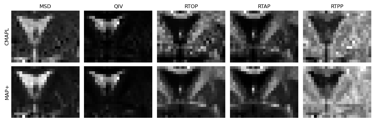
From now on we will just use the combined approach and the globally constrained approach, show all maps we can generate, and explain their significance.

fits = fits[2:]
fit_labels = fit_labels[2:]

compare_maps(
    fits,
    maps=["msd", "qiv", "rtop", "rtap", "rtpp"],
    fit_labels=fit_labels,
    map_labels=["MSD", "QIV", "RTOP", "RTAP", "RTPP"],
    filename="MAPMRI_maps.png",
)

From left to right:

• Mean squared displacement (MSD) is a measure for how far protons are able to diffuse. a decrease in MSD indicates protons are hindered/restricted more, as can be seen by the high MSD in the CSF, but low in the white matter.

• Q-space Inverse Variance (QIV) is a measure of variance in the signal, which is said to have higher contrast to white matter than the MSD [5]. QIV has also been shown to have high sensitivity to tissue composition change in a simulation study [6].

• Return-to-origin probability (RTOP) quantifies the probability that a proton will be at the same position at the first and second diffusion gradient pulse. A higher RTOP indicates that the volume a spin is inside of is smaller, meaning more overall restriction. This is illustrated by the low values in CSF and high values in white matter.

• Return-to-axis probability (RTAP) is a directional index that quantifies the probability that a proton will be along the axis of the main eigenvector of a diffusion tensor during both diffusion gradient pulses. RTAP has been related to the apparent axon diameter [1], [3] under several strong assumptions on the tissue composition and acquisition protocol.

• Return-to-plane probability (RTPP) is a directional index that quantifies the probability that a proton will be on the plane perpendicular to the main eigenvector of a diffusion tensor during both gradient pulses. RTPP is related to the length of a pore [1] but in practice should be similar to that of Gaussian diffusion.

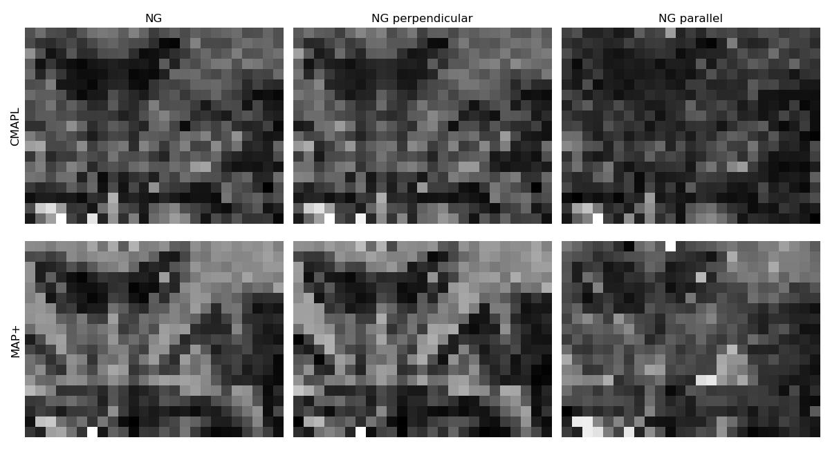
It is also possible to estimate the amount of non-Gaussian diffusion in every voxel [1]. This quantity is estimated through the ratio between Gaussian volume (MAP-MRI’s first basis function) and the non-Gaussian volume (all other basis functions) of the fitted signal. For this value to be physically meaningful we must use a b-value threshold in the MAP-MRI model. This threshold makes the scale estimation in MAP-MRI use only samples that realistically describe Gaussian diffusion, i.e., at low b-values.

map_model_both_ng = mapmri.MapmriModel(
    gtab,
    radial_order=radial_order,
    laplacian_regularization=True,
    laplacian_weighting=0.05,
    positivity_constraint=True,
    bval_threshold=2000,
)

map_model_plus_ng = mapmri.MapmriModel(
    gtab,
    radial_order=radial_order,
    positivity_constraint=True,
    global_constraints=True,
    bval_threshold=2000,
)

mapfit_both_ng = map_model_both_ng.fit(data_small)
mapfit_plus_ng = map_model_plus_ng.fit(data_small)

fits = [mapfit_both_ng, mapfit_plus_ng]
fit_labels = ["CMAPL", "MAP+"]

compare_maps(
    fits,
    maps=["ng", "ng_perpendicular", "ng_parallel"],
    fit_labels=fit_labels,
    map_labels=["NG", "NG perpendicular", "NG parallel"],
    filename="MAPMRI_ng.png",
)

On the left we see the overall NG and on the right the directional perpendicular NG and parallel NG. The NG ranges from 1 (completely non-Gaussian) to 0 (completely Gaussian). The overall NG of a voxel is always higher or equal than each of its components. It can be seen that NG has low values in the CSF and higher in the white matter.

Increases or decreases in these values do not point to a specific microstructural change, but can indicate clues as to what is happening, similar to fractional anisotropy. An initial simulation study that quantifies the added value of q-space indices over DTI indices is given in [6].

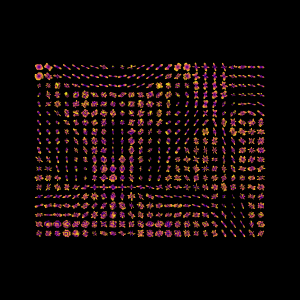
The MAP-MRI framework also allows for the estimation of orientation distribution functions (ODFs). We recommend to use the isotropic implementation for this purpose, as the anisotropic implementation has a bias towards smaller crossing angles.

For the isotropic basis we recommend to use a radial_order of 8, as the basis needs more generic and needs more basis functions to approximate the signal.

radial_order = 8
map_model_both_iso = mapmri.MapmriModel(
    gtab,
    radial_order=radial_order,
    laplacian_regularization=True,
    laplacian_weighting=0.1,
    positivity_constraint=True,
    anisotropic_scaling=False,
)

mapfit_both_iso = map_model_both_iso.fit(data_small)

Load an ODF reconstruction sphere.

sphere = get_sphere(name="repulsion724")

Compute the ODFs.

The radial order s can be increased to sharpen the results, but it might also make the ODFs noisier. Always check the results visually.

odf = mapfit_both_iso.odf(sphere, s=2)
print(f"odf.shape {odf.shape}")

odf.shape (25, 1, 19, 724)

Display the ODFs.

# Enables/disables interactive visualization
interactive = False

scene = window.Scene()
sfu = actor.odf_slicer(odf, sphere=sphere, colormap="plasma", scale=0.5)
sfu.display(y=0)
sfu.RotateX(-90)
scene.add(sfu)
window.record(scene=scene, out_path="odfs.png", size=(600, 600))
if interactive:
    window.show(scene)

Orientation distribution functions (ODFs).

References

[1] (1,2,3,4,5,6,7)

Evren Özarslan, Cheng Guan Koay, Timothy M. Shepherd, Michal E. Komlosh, M. Okan İrfanoǧlu, Carlo Pierpaoli, and Peter J. Basser. Mean apparent propagator (MAP) MRI: A novel diffusion imaging method for mapping tissue microstructure. NeuroImage, 78:16–32, 2013. URL: https://doi.org/10.1016/j.neuroimage.2013.04.016, doi:10.1016/j.neuroimage.2013.04.016.

[2] (1,2)

Tom Dela Haije, Evren Özarslan, and Aasa Feragen. Enforcing necessary non-negativity constraints for common diffusion MRI models using sum of squares programming. NeuroImage, 209:116405, 2020. URL: https://doi.org/10.1016/j.neuroimage.2019.116405, doi:10.1016/j.neuroimage.2019.116405.

[3] (1,2,3,4,5,6)

Rutger H. J. Fick, Demian Wassermann, Emmanuel Caruyer, and Rachid Deriche. MAPL: Tissue microstructure estimation using Laplacian-regularized MAP-MRI and its application to HCP data. NeuroImage, 134:365–385, July 2016. URL: https://doi.org/10.1016/j.neuroimage.2016.03.046, doi:10.1016/j.neuroimage.2016.03.046.

[4]

Peter Craven and Grace Wahba. Smoothing Noisy Data with Spline Functions - Estimating the Correct Degree of Smoothing by the Method of Generalized Cross-Validation. Numerische Mathematik, 31(4):377–403, 1979. doi:.

[5]

A. Pasha Hosseinbor, Moo K. Chung, Yu-Chien Wu, and Andrew L. Alexander. Bessel Fourier Orientation Reconstruction (BFOR): An analytical diffusion propagator reconstruction for hybrid diffusion imaging and computation of q-space indices. NeuroImage, 64:650–670, 2013. URL: https://doi.org/10.1016/j.neuroimage.2012.08.072, doi:10.1016/j.neuroimage.2012.08.072.

[6] (1,2)

Rutger H. J. Fick, MArco Pizzolato, Demian Wassermann, Mauro Zucchelli, Gloria Menegaz, and Rachid Deriche. A sensitivity analysis of q-space indices with respect to changes in axonal diameter, dispersion and tissue composition. In IEEE 13th International Symposium on Biomedical Imaging (ISBI), volume, 1241–1244. April 2016. doi:10.1109/ISBI.2016.7493491.