Reconstruction with the Sparse Fascicle Model (SFM)

In this example, we will use the Sparse Fascicle Model (SFM) [1], to reconstruct the fiber Orientation Distribution Function (fODF) in every voxel.

First, we import the modules we will use in this example:

from dipy.core.gradients import gradient_table
import dipy.data as dpd
import dipy.direction.peaks as dpp
from dipy.io.gradients import read_bvals_bvecs
from dipy.io.image import load_nifti
from dipy.reconst.csdeconv import auto_response_ssst
import dipy.reconst.sfm as sfm
from dipy.viz import actor, window

For the purpose of this example, we will use the Stanford HARDI dataset (150 directions, single b-value of 2000 \(s/mm^2\)) that can be automatically downloaded. If you have not yet downloaded this data-set in one of the other examples, you will need to be connected to the internet the first time you run this example. The data will be stored for subsequent runs, and for use with other examples.

hardi_fname, hardi_bval_fname, hardi_bvec_fname = dpd.get_fnames(name="stanford_hardi")
data, affine = load_nifti(hardi_fname)

bvals, bvecs = read_bvals_bvecs(hardi_bval_fname, hardi_bvec_fname)
gtab = gradient_table(bvals, bvecs=bvecs)

# Enables/disables interactive visualization
interactive = False

Reconstruction of the fiber ODF in each voxel guides subsequent tracking steps. Here, the model is the Sparse Fascicle Model, described in [1]. This model reconstructs the diffusion signal as a combination of the signals from different fascicles. This model can be written as:

\[y = X\beta\]

Where \(y\) is the signal and \(\beta\) are weights on different points in the sphere. The columns of the design matrix, \(X\) are the signals in each point in the measurement that would be predicted if there was a fascicle oriented in the direction represented by that column. Typically, the signal used for this kernel will be a prolate tensor with axial diffusivity 3-5 times higher than its radial diffusivity. The exact numbers can also be estimated from examining parts of the brain in which there is known to be only one fascicle (e.g. in corpus callosum).

Sparsity constraints on the fiber ODF (\(\beta\)) are set through the Elastic Net algorithm [2].

Elastic Net optimizes the following cost function:

\[\sum_{i=1}^{n}{(y_i - \hat{y}_i)^2} + \alpha (\lambda \sum_{j=1}^{m}{w_j}+(1-\lambda) \sum_{j=1}^{m}{w^2_j} # noqa: E501\]

where \(\hat{y}\) is the signal predicted for a particular setting of \(\beta\), such that the left part of this expression is the squared loss function; \(\alpha\) is a parameter that sets the balance between the squared loss on the data, and the regularization constraints. The regularization parameter \(\lambda\) sets the l1_ratio, which controls the balance between L1-sparsity (low sum of weights), and low L2-sparsity (low sum-of-squares of the weights).

Just like Constrained Spherical Deconvolution (see Reconstruction with Constrained Spherical Deconvolution model (CSD)), the SFM requires the definition of a response function. We’ll take advantage of the automated algorithm in the csdeconv module to find this response function:

response, ratio = auto_response_ssst(gtab, data, roi_radii=10, fa_thr=0.7)

The response return value contains two entries. The first is an array with the eigenvalues of the response function and the second is the average S0 for this response.

It is a very good practice to always validate the result of auto_response_ssst. For, this purpose we can print it and have a look at its values.

print(response)

(array([0.00139919, 0.0003007 , 0.0003007 ]), np.float64(416.7372408293461))

We initialize an SFM model object, using these values. We will use the default sphere (362 vertices, symmetrically distributed on the surface of the sphere), as a set of putative fascicle directions that are considered in the model

sphere = dpd.get_sphere()
sf_model = sfm.SparseFascicleModel(
    gtab, sphere=sphere, l1_ratio=0.5, alpha=0.001, response=response[0]
)

For the purpose of the example, we will consider a small volume of data containing parts of the corpus callosum and of the centrum semiovale

data_small = data[20:50, 55:85, 38:39]

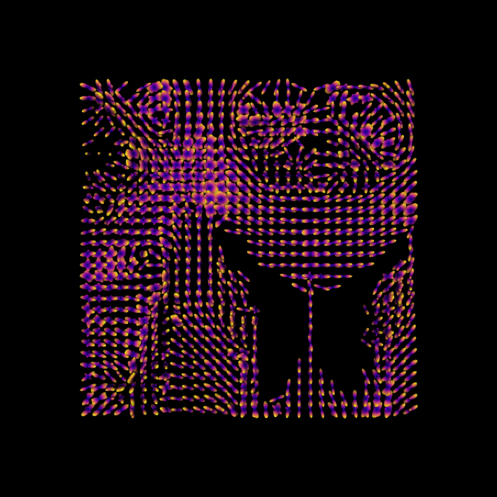
Fitting the model to this small volume of data, we calculate the ODF of this model on the sphere, and plot it.

sf_fit = sf_model.fit(data_small)
sf_odf = sf_fit.odf(sphere)

fodf_spheres = actor.odf_slicer(sf_odf, sphere=sphere, scale=0.8, colormap="plasma")

scene = window.Scene()
scene.add(fodf_spheres)

window.record(scene=scene, out_path="sf_odfs.png", size=(1000, 1000))
if interactive:
    window.show(scene)

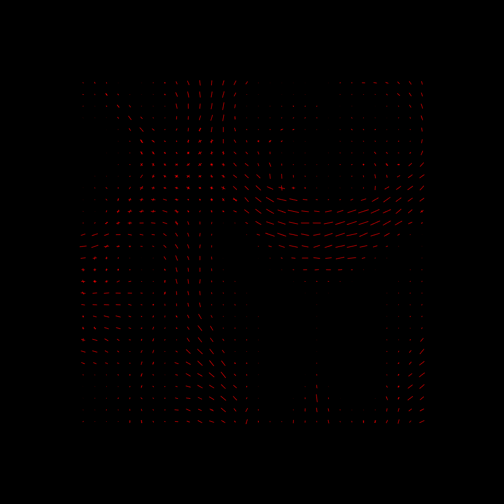
We can extract the peaks from the ODF, and plot these as well

sf_peaks = dpp.peaks_from_model(
    sf_model,
    data_small,
    sphere,
    relative_peak_threshold=0.5,
    min_separation_angle=25,
    return_sh=False,
)


scene.clear()
fodf_peaks = actor.peak_slicer(sf_peaks.peak_dirs, peaks_values=sf_peaks.peak_values)
scene.add(fodf_peaks)

window.record(scene=scene, out_path="sf_peaks.png", size=(1000, 1000))
if interactive:
    window.show(scene)

Finally, we plot both the peaks and the ODFs, overlaid:

fodf_spheres.GetProperty().SetOpacity(0.4)
scene.add(fodf_spheres)

window.record(scene=scene, out_path="sf_both.png", size=(1000, 1000))
if interactive:
    window.show(scene)

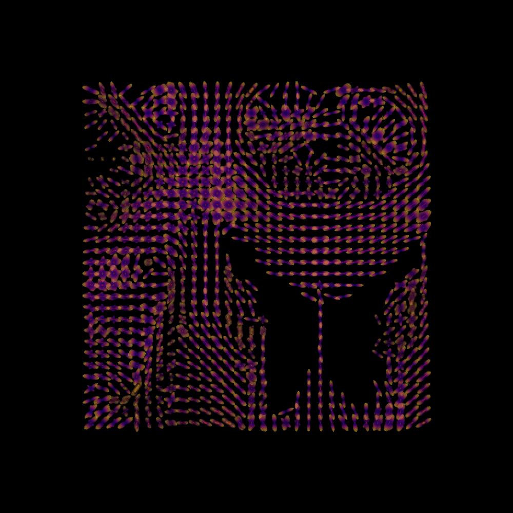
SFM Peaks and ODFs.

To see how to use this information in tracking, proceed to Tracking with the Sparse Fascicle Model.

References

[1] (1,2)

Ariel Rokem, Jason D. Yeatman, Franco Pestilli, Kendrick N. Kay, Aviv Mezer, Stefan van der Walt, and Brian A. Wandell. Evaluating the Accuracy of Diffusion MRI Models in White Matter. PLOS ONE, 10(4):1–26, April 2015. URL: https://doi.org/10.1371/journal.pone.0123272, doi:10.1371/journal.pone.0123272.

[2]

Hui Zou and Trevor Hastie. Regularization and Variable Selection Via the Elastic Net. Journal of the Royal Statistical Society Series B: Statistical Methodology, 67(2):301–320, March 2005. URL: https://doi.org/10.1111/j.1467-9868.2005.00503.x, doi:10.1111/j.1467-9868.2005.00503.x.