Reconstruction#
Below, an overview of all reconstruction models available in DIPY.
Note
Some reconstruction models do not have a tutorial yet
Method |
Single Shell |
Multi Shell |
Cartesian |
Paper Data Descriptions |
References |
|---|---|---|---|---|---|
Yes |
Yes |
Yes |
Typical b-value = 1000 s/mm^2, maximum b-value 1200 s/mm^2 (some success up to 1500 s/mm^2) |
Basser et al. [BMLeBihan94b] |
|
Yes |
Yes |
Yes |
Typical b-value = 1000 s/mm^2, maximum b-value 1200 s/mm^2 (some success up to 1500 s/mm^2) |
Chang et al. [CJP05], Chung et al. [CLH06], Yendiki et al. [YKK+14] |
|
No |
Yes |
No |
DTI-style acquisition, multiple b=0, all shells should be within maximum b-value of 1000 s/mm^2 (or 32 directions evenly distributed 500 s/mm^2 and 1500 s/mm^2 per Neto Henriques et al. [NetoHenriquesRG+17]) |
Pasternak et al. [PSG+09], Neto Henriques et al. [NetoHenriquesRG+17] |
|
No |
Yes |
No |
Dual spin echo diffusion-weighted 2D EPI images were acquired with b values of 0, 500, 1000, 1500, 2000, and 2500 s/mm^2 (max b value of 2000 suggested as sufficient in brain tissue); at least 15 directions |
Jensen et al. [JHR+05] |
|
No |
Yes |
No |
None |
Dela Haije et al. [DelaHaijeOzarslanF20] |
|
No |
Yes |
No |
DKI-style acquisition: at least two non-zero b shells (max b value 2000), minimum of 15 directions; typically b-values in increments of 500 from 0 to 2000, 30 directions |
||
No |
Yes |
No |
b-values in increments of 500 from 0 to 2000 s/mm^2, 30 directions |
Neto Henriques [NetoHenriques18] |
|
Yes |
No |
No |
HARDI data (preferably 7T) with at least 200 diffusion images at b=3000 s/mm^2, or multi-shell data with high angular resolution |
Aganj et al. [ALS+10] |
|
Westins CSA |
Yes |
No |
No |
||
No |
Yes |
No |
low b-values are needed |
Le Bihan et al. [LeBihanBL+88] |
|
No |
Yes |
No |
Fadnavis et al. [FRF+19] |
||
SDT |
Yes |
No |
No |
QBI-style acquisition (60-64 directions, b-value 1000 s/mm^2) |
Descoteaux et al. [DDKnoscheA09] |
No |
No |
Yes |
515 diffusion encodings, b-values from 12,000 to 18,000 s/mm^2. Acceleration in subsequent studies with ~100 diffusion encoding directions in half sphere of the q-space with b-values = 1000, 2000, 3000 s/mm^2) |
||
No |
No |
Yes |
203 diffusion encodings (isotropic 3D grid points in the q-space contained within a sphere with radius 3.6), maximum b-value = 4000 s/mm^2 |
Canales-Rodríguez et al. [CRodriguezIMAlemanGomezMGarcia10] |
|
No |
Yes |
Yes |
Fits any sampling scheme with at least one non-zero b-shell, benefits from more directions. Recommended 23 b-shells ranging from 0 to 4000 in a 258 direction grid-sampling scheme |
Yeh et al. [YWT10] |
|
Yes |
Yes |
No |
At least 40 directions, b-value above 1000 s/mm^2 |
Rokem et al. [RYP+15] |
|
Yes |
No |
No |
At least 64 directions, maximum b-values 3000-4000 s/mm^2, multi-shell, isotropic voxel size |
Tuch [Tuc04], Descoteaux et al. [DAFD07], Tristán-Vega et al. [TristanVAFernandezW09] |
|
No |
Yes |
No |
Multi-shell HARDI data (500, 1000, and 2000 s/mm^2; minimum 2 non-zero b-shells) or DSI (514 images in a cube of five lattice-units, one b=0) |
Merlet and Deriche [MD13], Özarslan et al. [OzarslanKB08], Özarslan et al. [OzarslanKS+09] |
|
No |
Yes |
No |
Six unit sphere shells with b = 1000, 2000, 3000, 4000, 5000, 6000 s/mm^2 along 19, 32, 56, 87, 125, and 170 directions (see Olson et al. [OAM19] for candidate sub-sampling schemes) |
Özarslan et al. [OzarslanKS+13], Olson et al. [OAM19] |
|
No |
Yes |
No |
Dela Haije et al. [DelaHaijeOzarslanF20] |
||
MAPL |
No |
Yes |
No |
Multi-shell similar to WU-Minn HCP, with minimum of 60 samples from 2 shells b-value 1000 and 3000 s/mm^2 |
Fick et al. [FWCD16] |
Yes |
No |
No |
Minimum: 20 gradient directions and a b-value of 1000 s/mm^2; benefits additionally from 60 direction HARDI data with b-value = 3000 s/mm^2 or multi-shell |
Tournier et al. [TCGC04], Tournier et al. [TCC07], Descoteaux et al. [DAFD07] |
|
No |
Yes |
No |
5 b=0, 50 directions at 3 non-zero b-shells: b=1000, 2000, 3000 s/mm^2 |
Jeurissen et al. [JTD+14] |
|
No |
Yes |
No |
Multi-shell 64 direction b-values of 1000, 2000 s/mm^2 as in Alexander et al. [AEA+17]. Original model used 1480 s/mm^2 with 92 directions and 36 b=0 |
||
Yes |
Yes |
Yes |
HARDI data with 64 directions at b = 2500 s/mm^2, 3 b=0 images (full original acquisition: 256 directions on a sphere at b = 2500 s/mm^2, 36 b=0 volumes) |
Canales-Rodríguez et al. [CRodriguezDS+15] |
|
No |
Yes |
No |
Evenly distributed geometric sampling scheme of 216 measurements, 5 b-values (50, 250, 50, 1000, 200 s/mm^2), measurement tensors of four shapes: stick, prolate, sphere, and plane |
Westin et al. [WKP+16] |
|
No |
Yes |
No |
At least one b=0, minimum of 39 acquisitions with spherical and linear encoding; optimal 120 (see Morez et al. [MSdenDekker+23]), ideal 217 see Table 1 in Herberthson et al. [HBH+21] |
Herberthson et al. [HBH+21], Morez et al. [MSdenDekker+23] |
|
Ball & Stick |
Yes |
Yes |
No |
Three b=0, 60 evenly distributed directions per Jones et al. [JHS99] at b-value 1000 s/mm^2 |
Behrens et al. [BWMJ+03] |
No |
Yes |
No |
Minimum 200 volumes of multi-spherical dMRI (multi-shell, multi-diffusion time; varying gradient directions, gradient strengths, and diffusion times) |
Fick et al. [FPS+18] |
|
Power Map |
Yes |
Yes |
No |
HARDI data with 60 directions at b-value = 3000 s/mm^2, 7 b=0 (Minimum: HARDI data with at least 30 directions) |
Dell'Acqua et al. [DellAcquaLCS14] |
No |
Yes |
No |
72 directions at each of 5 evenly spaced b-values from 0.5 to 2.5 ms/μm^2, 5 b-values from 3 to 5 ms/μm^2, 5 b-values from 5.5 to 7.5 ms/μm^2, and 3 b-values from 8 to 9 ms/μm^2 / b=0 ms/μm^2, and along 33 directions at b-values from 0.2–3 ms/μm^2 in steps of 0.2 ms/μm^2 (24 point spherical design and 9 directions identified for rapid kurtosis estimation) |
Kaden et al. [KKC+16], Neto Henriques et al. [NetoHenriquesJS19] |
|
No |
Yes |
No |
Neto Henriques et al. [NetoHenriquesJS20], Neto Henriques et al. [NetoHenriquesJS21], Novello et al. [NNetoHenriquesI+22] |

Applying positivity constraints to Q-space Trajectory Imaging (QTI+)

Reconstruction of the diffusion signal with the correlation tensor model (CTI)
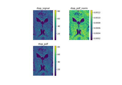
Continuous and analytical diffusion signal modelling with 3D-SHORE
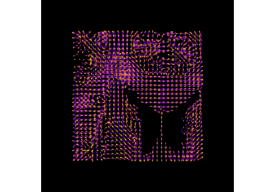
Reconstruction with the Sparse Fascicle Model (SFM)
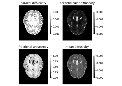
Crossing invariant fiber response function with FORECAST model
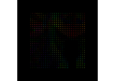
Reconstruction of the diffusion signal with DTI (single tensor) model
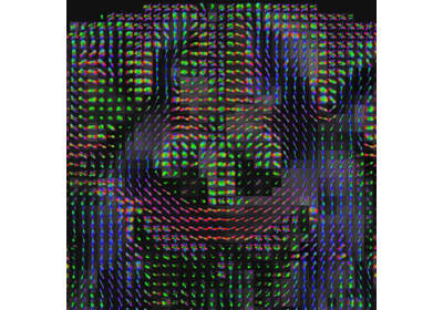
Local reconstruction using the Histological ResDNN
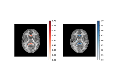
Reconstruction of the diffusion signal with the WMTI model (DKI-MICRO)
Using the RESTORE algorithm for robust tensor fitting
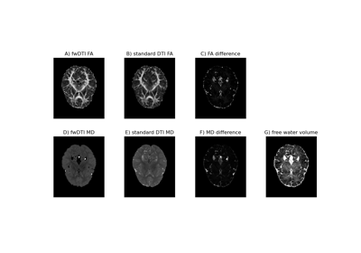
Using the free water elimination model to remove DTI free water contamination
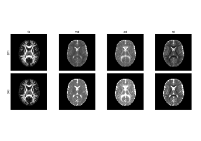
Reconstruction of the diffusion signal with the kurtosis tensor model (DKI)

Reconstruction with FORCE (FORward modeling for Complex microstructure Estimation)
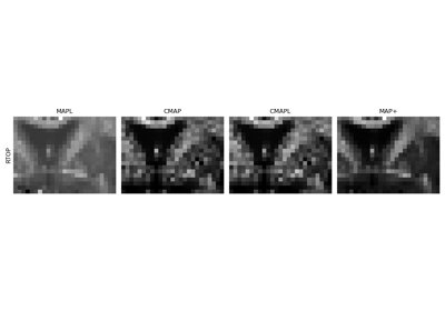
Continuous and analytical diffusion signal modelling with MAP-MRI
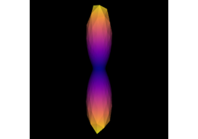
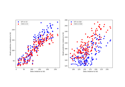
Reconstruction with Constrained Spherical Deconvolution model (CSD)
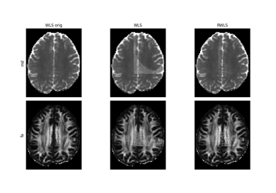
Robust fitting with iteratively reweighted least squares.
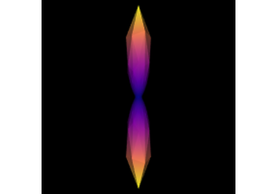
Reconstruction with Robust and Unbiased Model-BAsed Spherical Deconvolution (RUMBA)
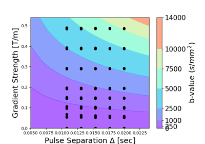
Estimating diffusion time dependent q-space indices using qt-dMRI
