Continuous and analytical diffusion signal modelling with 3D-SHORE

We show how to model the diffusion signal as a linear combination of continuous functions from the SHORE basis [Merlet2013], [Özarslan2008], [Özarslan2009]. We also compute the analytical Orientation Distribution Function (ODF).

First import the necessary modules:

from dipy.reconst.shore import ShoreModel
from dipy.viz import window, actor
from dipy.core.gradients import gradient_table
from dipy.data import get_fnames, get_sphere
from dipy.io.gradients import read_bvals_bvecs
from dipy.io.image import load_nifti

Download and read the data for this tutorial.

# ``fetch_isbi2013_2shell()`` provides data from the `ISBI HARDI contest 2013
# <http://hardi.epfl.ch/static/events/2013_ISBI/>`_ acquired for two shells at
# b-values 1500 :math:`s/mm^2` and 2500 :math:`s/mm^2`.

# The six parameters of these two functions define the ROI where to reconstruct
# the data. They respectively correspond to ``(xmin,xmax,ymin,ymax,zmin,zmax)``
# with x, y, z and the three axis defining the spatial positions of the voxels.

fraw, fbval, fbvec = get_fnames('isbi2013_2shell')

data, affine = load_nifti(fraw)
bvals, bvecs = read_bvals_bvecs(fbval, fbvec)
gtab = gradient_table(bvals, bvecs)
data_small = data[10:40, 22, 10:40]

print('data.shape (%d, %d, %d, %d)' % data.shape)

data.shape (50, 50, 50, 64)

data contains the voxel data and gtab contains a GradientTable object (gradient information e.g. b-values). For example, to show the b-values it is possible to write:

print(gtab.bvals)

Instantiate the SHORE Model.

radial_order is the radial order of the SHORE basis.

zeta is the scale factor of the SHORE basis.

lambdaN and lambdaL are the radial and angular regularization constants, respectively.

For details regarding these four parameters see [Cheng2011] and [Merlet2013].

radial_order = 6
zeta = 700
lambdaN = 1e-8
lambdaL = 1e-8
asm = ShoreModel(gtab, radial_order=radial_order,
                 zeta=zeta, lambdaN=lambdaN, lambdaL=lambdaL)

Fit the SHORE model to the data

asmfit = asm.fit(data_small)

  0%|                                                                                                                                           | 0/900 [00:00<?, ?it/s]
 23%|█████████████████████████████▋                                                                                                 | 210/900 [00:00<00:00, 2087.41it/s]
 49%|█████████████████████████████████████████████████████████████▋                                                                 | 437/900 [00:00<00:00, 2190.34it/s]
 74%|██████████████████████████████████████████████████████████████████████████████████████████████                                 | 667/900 [00:00<00:00, 2236.68it/s]
100%|███████████████████████████████████████████████████████████████████████████████████████████████████████████████████████████████| 900/900 [00:00<00:00, 2245.92it/s]

Load an odf reconstruction sphere

sphere = get_sphere('repulsion724')

Compute the ODFs

odf = asmfit.odf(sphere)
print('odf.shape (%d, %d, %d)' % odf.shape)

odf.shape (30, 30, 724)

Display the ODFs

# Enables/disables interactive visualization
interactive = False

scene = window.Scene()
sfu = actor.odf_slicer(odf[:, None, :], sphere=sphere, colormap='plasma',
                       scale=0.5)
sfu.RotateX(-90)
sfu.display(y=0)
scene.add(sfu)
window.record(scene, out_path='odfs.png', size=(600, 600))
if interactive:
    window.show(scene)

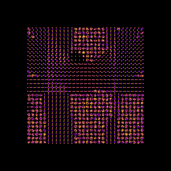
Orientation distribution functions.

References

[Özarslan2008]

Özarslan E. et al., “Simple harmonic oscillator based estimation and reconstruction for one-dimensional q-space MR,” in Proc Intl Soc Mag Reson Med, 16, Toronto, Canada, 2008

[Özarslan2009]

Özarslan E. et al., “Simple harmonic oscillator based reconstruction and estimation for three-dimensional q-space MRI,” in Proc Intl Soc Mag Reson Med, 17, Honolulu, HI, 2009

[Merlet2013] (1,2)

Merlet S. et al., “Continuous diffusion signal, EAP and ODF estimation via Compressive Sensing in diffusion MRI”, Medical Image Analysis, 2013.

[Cheng2011]

Cheng J. et al., “Theoretical Analysis and Practical Insights on EAP Estimation via Unified HARDI Framework”, MICCAI workshop on Computational Diffusion MRI, 2011.