Patch2Self: Self-Supervised Denoising via Statistical Independence

Patch2Self [Fadnavis20] is a self-supervised learning method for denoising DWI data, which uses the entire volume to learn a full-rank locally linear denoiser for that volume. By taking advantage of the oversampled q-space of DWI data, Patch2Self can separate structure from noise without requiring an explicit model for either.

Classical denoising algorithms such as Local PCA [Manjon2013], [Veraa2016a], Non-local Means [Coupe08], Total Variation Norm [Knoll11], etc. assume certain properties on the signal structure. Patch2Self does not make any such assumption on the signal, instead using the fact that the noise across different 3D volumes of the DWI signal originates from random fluctuations in the acquired signal.

Since Patch2Self only relies on the randomness of the noise, it can be applied at any step in the pre-processing pipeline. The design of Patch2Self is such that it can work on any type of diffusion data/ any body part without requiring a noise estimation or assumptions on the type of noise (such as its distribution).

The Patch2Self Framework:

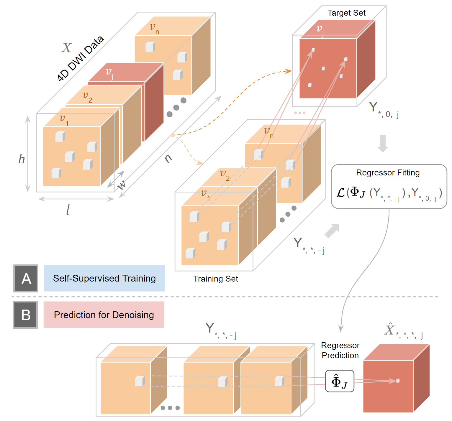
The above figure demonstrates the working of Patch2Self. The idea is to build a new regressor for denoising each 3D volume of the 4D diffusion data. This is done in the following 2 phases:

(A) Self-supervised training: First, we extract 3D Patches from all the n volumes and hold out the target volume to denoise. Each patch from the rest of the (n-1) volumes predicts the center voxel of the corresponding patch in the target volume.

This is done by using the self-supervised loss:

\[\mathcal{L}\left(\Phi_{J}\right)=\mathbb{E}\left\|\Phi_{J}\ \left(Y_{*, *,-j}\right)-Y_{*, 0, j}\right\|^{2}\]

(B) Prediction: The same ‘n-1’ volumes which were used in the training are now fed into the regressor \(\Phi\) built in phase (A). The prediction is a denoised version of held-out volume.

Note: The volume to be denoised is merely used as the target in the training phase. But is not used in the training set for (A) nor is used to predict the denoised output in (B).

Let’s load the necessary modules:

import numpy as np
from dipy.data import get_fnames
from dipy.io.image import load_nifti, save_nifti
import matplotlib.pyplot as plt

from dipy.denoise.patch2self import patch2self

Now let’s load an example dataset and denoise it with Patch2Self. Patch2Self does not require noise estimation and should work with any kind of diffusion data.

hardi_fname, hardi_bval_fname, hardi_bvec_fname = get_fnames('stanford_hardi')
data, affine = load_nifti(hardi_fname)
bvals = np.loadtxt(hardi_bval_fname)
denoised_arr = patch2self(data, bvals, model='ols', shift_intensity=True,
                          clip_negative_vals=False, b0_threshold=50)

The above parameters should give optimal denoising performance for Patch2Self. The ordinary least squares regression (model='ols') tends to be a little slower depending on the size of the data. In that case, please consider switching to ridge regression (model='ridge').

Please do note that sometimes using ridge regression can hamper the performance of Patch2Self. If so, please use model='ols'.

The array denoised_arr contains the denoised output obtained from Patch2Self.

Depending on the acquisition, b0 may exhibit signal attenuation or other artefacts that are not ideal for any denoising algorithm. We therefore provide an option to skip denoising b0 volumes in the data. This can be done by using the option b0_denoising=False within Patch2Self.

Please set shift_intensity=True and clip_negative_vals=False by default to avoid negative values in the denoised output.

The b0_threshold is used to separate the b0 volumes from the DWI volumes. Changing the value of the b0 threshold is needed if the b0 volumes in the bval file have a value greater than the default b0_threshold.

The default value of b0_threshold in DIPY is set to 50. If using data such as HCP 7T, the b0 volumes tend to have a higher b-value (>=50) associated with them in the bval file. Please check the b-values for b0s and adjust the b0_threshold` accordingly.

Now let’s visualize the output and the residuals obtained from the denoising.

# Gets the center slice and the middle volume of the 4D diffusion data.
sli = data.shape[2] // 2
gra = 60  # pick out a random volume for a particular gradient direction

orig = data[:, :, sli, gra]
den = denoised_arr[:, :, sli, gra]

# computes the residuals
rms_diff = np.sqrt((orig - den) ** 2)

fig1, ax = plt.subplots(1, 3, figsize=(12, 6),
                        subplot_kw={'xticks': [], 'yticks': []})

fig1.subplots_adjust(hspace=0.3, wspace=0.05)

ax.flat[0].imshow(orig.T, cmap='gray', interpolation='none',
                  origin='lower')
ax.flat[0].set_title('Original')
ax.flat[1].imshow(den.T, cmap='gray', interpolation='none',
                  origin='lower')
ax.flat[1].set_title('Denoised Output')
ax.flat[2].imshow(rms_diff.T, cmap='gray', interpolation='none',
                  origin='lower')
ax.flat[2].set_title('Residuals')

fig1.savefig('denoised_patch2self.png')

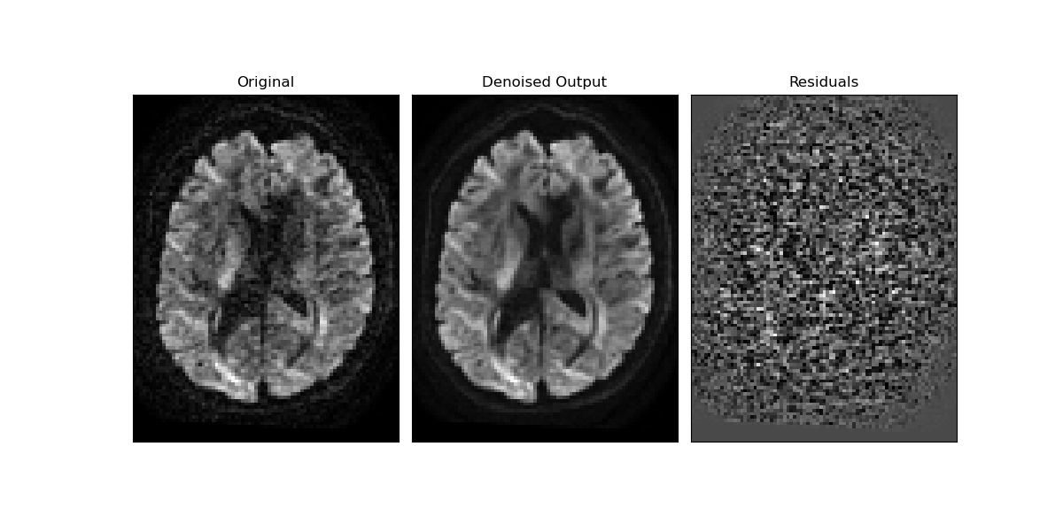
Patch2Self preserved anatomical detail. This can be visually verified by inspecting the residuals obtained above. Since we do not see any structure in the difference residuals, it is clear that it preserved the underlying signal structure and got rid of the stochastic noise.

Below we show how the denoised data can be saved.

save_nifti('denoised_patch2self.nii.gz', denoised_arr, affine)

Lastly, one can also use Patch2Self in batches if the number of gradient directions is very high (>=200 volumes). For instance, if the data has 300 volumes, one can split the data into 2 batches, (150 directions each) and still get the same denoising performance. One can run Patch2Self using:

denoised_batch1 = patch2self(data[..., :150], bvals[:150])
denoised_batch2 = patch2self(data[..., 150:], bvals[150:])

After doing this, the 2 denoised batches can be merged as follows:

denoised_p2s = np.concatenate((denoised_batch1, denoised_batch2), axis=3)

One can also consider using the above batching approach to denoise each shell separately if working with multi-shell data.

References

[Fadnavis20]

S. Fadnavis, J. Batson, E. Garyfallidis, Patch2Self: Denoising Diffusion MRI with Self-supervised Learning, Advances in Neural Information Processing Systems 33 (2020)

[Manjon2013]

Manjon JV, Coupe P, Concha L, Buades A, Collins DL “Diffusion Weighted Image Denoising Using Overcomplete Local PCA” (2013) PLoS ONE 8(9): e73021. doi:10.1371/journal.pone.0073021.

[Veraa2016a]

Veraart J, Fieremans E, Novikov DS. 2016. Diffusion MRI noise mapping using random matrix theory. Magnetic Resonance in Medicine. doi: 10.1002/mrm.26059.

[Coupe08]

P. Coupe, P. Yger, S. Prima, P. Hellier, C. Kervrann, C. Barillot, An Optimized Blockwise Non Local Means Denoising Filter for 3D Magnetic Resonance Images, IEEE Transactions on Medical Imaging, 27(4):425-441, 2008

[Knoll11]

F. Knoll, K. Bredies, T. Pock, R. Stollberger, Second order total generalized variation (TGV) for MRI. Magnetic resonance in medicine, 65(2), pp.480-491.