Reconstruction of the diffusion signal with the Tensor model

The diffusion tensor model is a model that describes the diffusion within a voxel. First proposed by Basser and colleagues [Basser1994], it has been very influential in demonstrating the utility of diffusion MRI in characterizing the micro-structure of white matter tissue and of the biophysical properties of tissue, inferred from local diffusion properties and it is still very commonly used.

The diffusion tensor models the diffusion signal as:

\[\frac{S(\mathbf{g}, b)}{S_0} = e^{-b\mathbf{g}^T \mathbf{D} \mathbf{g}}\]

Where \(\mathbf{g}\) is a unit vector in 3 space indicating the direction of measurement and b are the parameters of measurement, such as the strength and duration of diffusion-weighting gradient. \(S(\mathbf{g}, b)\) is the diffusion-weighted signal measured and \(S_0\) is the signal conducted in a measurement with no diffusion weighting. \(\mathbf{D}\) is a positive-definite quadratic form, which contains six free parameters to be fit. These six parameters are:

\[\begin{split}\mathbf{D} = \begin{pmatrix} D_{xx} & D_{xy} & D_{xz} \\ D_{yx} & D_{yy} & D_{yz} \\ D_{zx} & D_{zy} & D_{zz} \\ \end{pmatrix}\end{split}\]

This matrix is a variance/covariance matrix of the diffusivity along the three spatial dimensions. Note that we can assume that diffusivity has antipodal symmetry, so elements across the diagonal are equal. For example: \(D_{xy} = D_{yx}\). This is why there are only 6 free parameters to estimate here.

In the following example we show how to reconstruct your diffusion datasets using a single tensor model.

First import the necessary modules:

numpy is for numerical computation

import numpy as np

dipy.io.image is for loading / saving imaging datasets dipy.io.gradients is for loading / saving our bvals and bvecs

from dipy.io.image import load_nifti, save_nifti
from dipy.io.gradients import read_bvals_bvecs
from dipy.core.gradients import gradient_table

dipy.reconst is for the reconstruction algorithms which we use to create voxel models from the raw data.

import dipy.reconst.dti as dti

dipy.data is used for small datasets that we use in tests and examples.

from dipy.data import get_fnames

get_fnames will download the raw dMRI dataset of a single subject. The size of the dataset is 87 MBytes. You only need to fetch once. It will return the file names of our data.

hardi_fname, hardi_bval_fname, hardi_bvec_fname = get_fnames('stanford_hardi')

Next, we read the saved dataset. gtab contains a GradientTable object (information about the gradients e.g. b-values and b-vectors).

data, affine = load_nifti(hardi_fname)

bvals, bvecs = read_bvals_bvecs(hardi_bval_fname, hardi_bvec_fname)
gtab = gradient_table(bvals, bvecs)

print('data.shape (%d, %d, %d, %d)' % data.shape)

data.shape (81, 106, 76, 160)

data.shape (81, 106, 76, 160)

First of all, we mask and crop the data. This is a quick way to avoid calculating Tensors on the background of the image. This is done using DIPY’s mask module.

from dipy.segment.mask import median_otsu

maskdata, mask = median_otsu(data, vol_idx=range(10, 50), median_radius=3,
                             numpass=1, autocrop=True, dilate=2)
print('maskdata.shape (%d, %d, %d, %d)' % maskdata.shape)

maskdata.shape (71, 88, 62, 160)

maskdata.shape (72, 87, 59, 160)

Now that we have prepared the datasets we can go forward with the voxel reconstruction. First, we instantiate the Tensor model in the following way.

tenmodel = dti.TensorModel(gtab)

Fitting the data is very simple. We just need to call the fit method of the TensorModel in the following way:

tenfit = tenmodel.fit(maskdata)

The fit method creates a TensorFit object which contains the fitting parameters and other attributes of the model. You can recover the 6 values of the triangular matrix representing the tensor D. By default, in DIPY, values are ordered as (Dxx, Dxy, Dyy, Dxz, Dyz, Dzz). The tensor_vals variable defined below is a 4D data with last dimension of size 6.

tensor_vals = dti.lower_triangular(tenfit.quadratic_form)

You can also recover other metrics from the model. For example we can generate fractional anisotropy (FA) from the eigen-values of the tensor. FA is used to characterize the degree to which the distribution of diffusion in a voxel is directional. That is, whether there is relatively unrestricted diffusion in one particular direction.

Mathematically, FA is defined as the normalized variance of the eigen-values of the tensor:

\[FA = \sqrt{\frac{1}{2}\frac{(\lambda_1-\lambda_2)^2+(\lambda_1- \lambda_3)^2+(\lambda_2-\lambda_3)^2}{\lambda_1^2+ \lambda_2^2+\lambda_3^2}}\]

Note that FA should be interpreted carefully. It may be an indication of the density of packing of fibers in a voxel, and the amount of myelin wrapping these axons, but it is not always a measure of “tissue integrity”. For example, FA may decrease in locations in which there is fanning of white matter fibers, or where more than one population of white matter fibers crosses.

print('Computing anisotropy measures (FA, MD, RGB)')
from dipy.reconst.dti import fractional_anisotropy, color_fa

FA = fractional_anisotropy(tenfit.evals)

Computing anisotropy measures (FA, MD, RGB)

In the background of the image the fitting will not be accurate there is no signal and possibly we will find FA values with nans (not a number). We can easily remove these in the following way.

FA[np.isnan(FA)] = 0

Saving the FA images is very easy using nibabel. We need the FA volume and the affine matrix which transform the image’s coordinates to the world coordinates. Here, we choose to save the FA in float32.

save_nifti('tensor_fa.nii.gz', FA.astype(np.float32), affine)

You can now see the result with any nifti viewer or check it slice by slice using matplotlib’s imshow. In the same way you can save the eigen values, the eigen vectors or any other properties of the tensor.

save_nifti('tensor_evecs.nii.gz', tenfit.evecs.astype(np.float32), affine)

Other tensor statistics can be calculated from the tenfit object. For example, a commonly calculated statistic is the mean diffusivity (MD). This is simply the mean of the eigenvalues of the tensor. Since FA is a normalized measure of variance and MD is the mean, they are often used as complimentary measures. In DIPY, there are two equivalent ways to calculate the mean diffusivity. One is by calling the mean_diffusivity module function on the eigen-values of the TensorFit class instance:

MD1 = dti.mean_diffusivity(tenfit.evals)
save_nifti('tensors_md.nii.gz', MD1.astype(np.float32), affine)

The other is to call the TensorFit class method:

MD2 = tenfit.md

Obviously, the quantities are identical.

We can also compute the colored FA or RGB-map [Pajevic1999]. First, we make sure that the FA is scaled between 0 and 1, we compute the RGB map and save it.

FA = np.clip(FA, 0, 1)
RGB = color_fa(FA, tenfit.evecs)
save_nifti('tensor_rgb.nii.gz', np.array(255 * RGB, 'uint8'), affine)

Let’s try to visualize the tensor ellipsoids of a small rectangular area in an axial slice of the splenium of the corpus callosum (CC).

print('Computing tensor ellipsoids in a part of the splenium of the CC')

from dipy.data import get_sphere
sphere = get_sphere('repulsion724')

from dipy.viz import window, actor

# Enables/disables interactive visualization
interactive = False

scene = window.Scene()

evals = tenfit.evals[13:43, 44:74, 28:29]
evecs = tenfit.evecs[13:43, 44:74, 28:29]

Computing tensor ellipsoids in a part of the splenium of the CC

We can color the ellipsoids using the color_fa values that we calculated above. In this example we additionally normalize the values to increase the contrast.

cfa = RGB[13:43, 44:74, 28:29]
cfa /= cfa.max()

scene.add(actor.tensor_slicer(evals, evecs, scalar_colors=cfa, sphere=sphere,
                              scale=0.3))

print('Saving illustration as tensor_ellipsoids.png')
window.record(scene, n_frames=1, out_path='tensor_ellipsoids.png',
              size=(600, 600))
if interactive:
    window.show(scene)

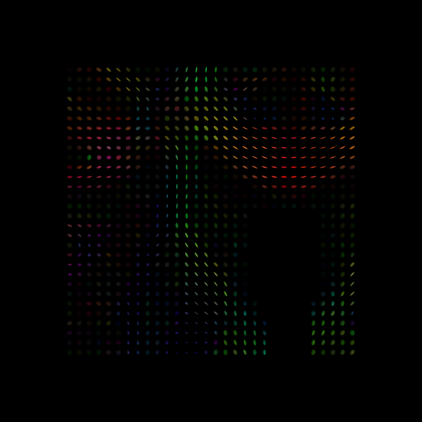
Saving illustration as tensor_ellipsoids.png

Tensor Ellipsoids.

scene.clear()

Finally, we can visualize the tensor Orientation Distribution Functions for the same area as we did with the ellipsoids.

tensor_odfs = tenmodel.fit(data[20:50, 55:85, 38:39]).odf(sphere)

odf_actor = actor.odf_slicer(tensor_odfs, sphere=sphere, scale=0.5,
                             colormap=None)
scene.add(odf_actor)
print('Saving illustration as tensor_odfs.png')
window.record(scene, n_frames=1, out_path='tensor_odfs.png', size=(600, 600))
if interactive:
    window.show(scene)

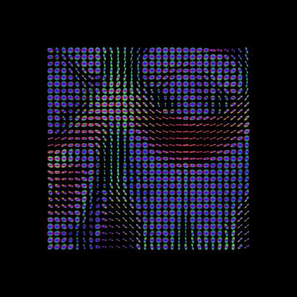
Saving illustration as tensor_odfs.png

Tensor ODFs.

Note that while the tensor model is an accurate and reliable model of the diffusion signal in the white matter, it has the drawback that it only has one principal diffusion direction. Therefore, in locations in the brain that contain multiple fiber populations crossing each other, the tensor model may indicate that the principal diffusion direction is intermediate to these directions. Therefore, using the principal diffusion direction for tracking in these locations may be misleading and may lead to errors in defining the tracks. Fortunately, other reconstruction methods can be used to represent the diffusion and fiber orientations in those locations. These are presented in other examples.

References

[Basser1994]

Basser PJ, Mattielo J, LeBihan (1994). MR diffusion tensor spectroscopy and imaging.

[Pajevic1999]

Pajevic S, Pierpaoli (1999). Color schemes to represent the orientation of anisotropic tissues from diffusion tensor data: application to white matter fiber tract mapping in the human brain.