Connectivity Matrices, ROI Intersections and Density Maps

This example is meant to be an introduction to some of the streamline tools available in DIPY. Some of the functions covered in this example are target, connectivity_matrix and density_map. target allows one to filter streamlines that either pass through or do not pass through some region of the brain, connectivity_matrix groups and counts streamlines based on where in the brain they begin and end, and finally, density map counts the number of streamlines that pass through every voxel of some image.

To get started we’ll need to have a set of streamlines to work with. We’ll use EuDX along with the CsaOdfModel to make some streamlines. Let’s import the modules and download the data we’ll be using.

Let’s load the necessary modules:

import numpy as np
import matplotlib.pyplot as plt
from scipy.ndimage import binary_dilation

from dipy.core.gradients import gradient_table
from dipy.data import get_fnames
from dipy.io.gradients import read_bvals_bvecs
from dipy.io.image import load_nifti_data, load_nifti, save_nifti
from dipy.io.stateful_tractogram import Space, StatefulTractogram
from dipy.io.streamline import save_trk
from dipy.direction import peaks
from dipy.reconst import shm
from dipy.tracking import utils
from dipy.tracking.local_tracking import LocalTracking
from dipy.tracking.stopping_criterion import BinaryStoppingCriterion
from dipy.tracking.streamline import Streamlines
from dipy.viz import window, actor, colormap as cmap

We’ll be using the Stanford HARDI dataset which consists of a single subject’s diffusion, b-values and b-vectors, T1 image and some labels in the same space as the T1. We’ll use the get_fnames function to download the files we need and set the file names to variables.

hardi_fname, hardi_bval_fname, hardi_bvec_fname = get_fnames('stanford_hardi')
label_fname = get_fnames('stanford_labels')
t1_fname = get_fnames('stanford_t1')

data, affine, hardi_img = load_nifti(hardi_fname, return_img=True)
labels = load_nifti_data(label_fname)
t1_data = load_nifti_data(t1_fname)
bvals, bvecs = read_bvals_bvecs(hardi_bval_fname, hardi_bvec_fname)
gtab = gradient_table(bvals, bvecs)

We’ve loaded an image called labels_img which is a map of tissue types such that every integer value in the array labels represents an anatomical structure or tissue type [1]. For this example, the image was created so that white matter voxels have values of either 1 or 2. We’ll use peaks_from_model to apply the CsaOdfModel to each white matter voxel and estimate fiber orientations which we can use for tracking. We will also dilate this mask by 1 voxel to ensure streamlines reach the grey matter.

white_matter = binary_dilation((labels == 1) | (labels == 2))
csamodel = shm.CsaOdfModel(gtab, 6)
csapeaks = peaks.peaks_from_model(model=csamodel,
                                  data=data,
                                  sphere=peaks.default_sphere,
                                  relative_peak_threshold=.8,
                                  min_separation_angle=45,
                                  mask=white_matter)

Now we can use EuDX to track all of the white matter. To keep things reasonably fast we use density=1 which will result in 1 seeds per voxel. The stopping criterion, determining when the tracking stops, is set to stop when the tracking exits the white matter.

affine = np.eye(4)
seeds = utils.seeds_from_mask(white_matter, affine, density=1)
stopping_criterion = BinaryStoppingCriterion(white_matter)

streamline_generator = LocalTracking(csapeaks, stopping_criterion, seeds,
                                     affine=affine, step_size=0.5)
streamlines = Streamlines(streamline_generator)

The first of the tracking utilities we’ll cover here is target. This function takes a set of streamlines and a region of interest (ROI) and returns only those streamlines that pass through the ROI. The ROI should be an array such that the voxels that belong to the ROI are True and all other voxels are False (this type of binary array is sometimes called a mask). This function can also exclude all the streamlines that pass through an ROI by setting the include flag to False. In this example we’ll target the streamlines of the corpus callosum. Our labels array has a sagittal slice of the corpus callosum identified by the label value 2. We’ll create an ROI mask from that label and create two sets of streamlines, those that intersect with the ROI and those that don’t.

cc_slice = labels == 2
cc_streamlines = utils.target(streamlines, affine, cc_slice)
cc_streamlines = Streamlines(cc_streamlines)

other_streamlines = utils.target(streamlines, affine, cc_slice,
                                 include=False)
other_streamlines = Streamlines(other_streamlines)
assert len(other_streamlines) + len(cc_streamlines) == len(streamlines)

We can use some of DIPY’s visualization tools to display the ROI we targeted above and all the streamlines that pass through that ROI. The ROI is the yellow region near the center of the axial image.

# Enables/disables interactive visualization
interactive = False

# Make display objects
color = cmap.line_colors(cc_streamlines)
cc_streamlines_actor = actor.line(cc_streamlines,
                                  cmap.line_colors(cc_streamlines))
cc_ROI_actor = actor.contour_from_roi(cc_slice, color=(1., 1., 0.),
                                      opacity=0.5)

vol_actor = actor.slicer(t1_data)

vol_actor.display(x=40)
vol_actor2 = vol_actor.copy()
vol_actor2.display(z=35)

# Add display objects to canvas
scene = window.Scene()
scene.add(vol_actor)
scene.add(vol_actor2)
scene.add(cc_streamlines_actor)
scene.add(cc_ROI_actor)

# Save figures
window.record(scene, n_frames=1, out_path='corpuscallosum_axial.png',
              size=(800, 800))
if interactive:
    window.show(scene)
scene.set_camera(position=[-1, 0, 0], focal_point=[0, 0, 0], view_up=[0, 0, 1])
window.record(scene, n_frames=1, out_path='corpuscallosum_sagittal.png',
              size=(800, 800))
if interactive:
    window.show(scene)

• 
• 

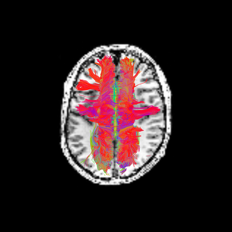
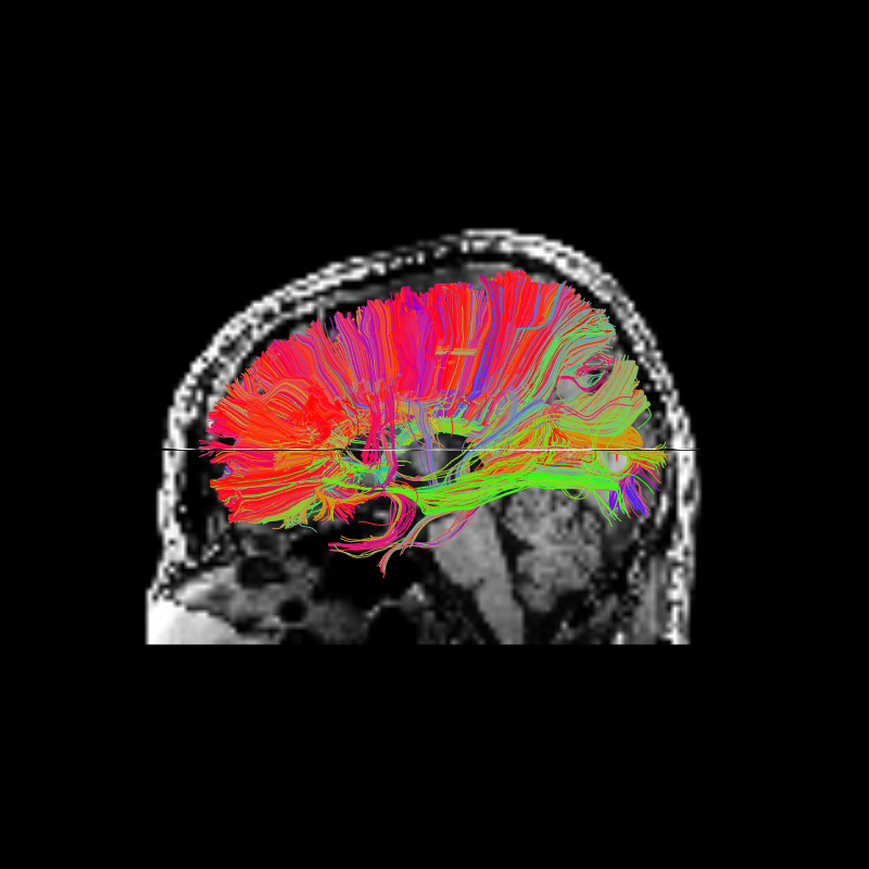
Corpus Callosum Axial and Corpus Callosum Sagittal

Once we’ve targeted the corpus callosum ROI, we might want to find out which regions of the brain are connected by these streamlines. To do this we can use the connectivity_matrix function. This function takes a set of streamlines and an array of labels as arguments. It returns the number of streamlines that start and end at each pair of labels and it can return the streamlines grouped by their endpoints. Notice that this function only considers the endpoints of each streamline.

M, grouping = utils.connectivity_matrix(cc_streamlines, affine,
                                        labels.astype(np.uint8),
                                        return_mapping=True,
                                        mapping_as_streamlines=True)
M[:3, :] = 0
M[:, :3] = 0

We’ve set return_mapping and mapping_as_streamlines to True so that connectivity_matrix returns all the streamlines in cc_streamlines grouped by their endpoint.

Because we’re typically only interested in connections between gray matter regions, and because the label 0 represents background and the labels 1 and 2 represent white matter, we discard the first three rows and columns of the connectivity matrix.

We can now display this matrix using matplotlib. We display it using a log scale to make small values in the matrix easier to see.

plt.imshow(np.log1p(M), interpolation='nearest')
plt.savefig("connectivity.png")

Connectivity of Corpus Callosum

In our example track there are more streamlines connecting regions 11 and 54 than any other pair of regions. These labels represent the left and right superior frontal gyrus respectively. These two regions are large, close together, have lots of corpus callosum fibers and are easy to track so this result should not be a surprise to anyone.

However, the interpretation of streamline counts can be tricky. The relationship between the underlying biology and the streamline counts will depend on several factors, including how the tracking was done, and the correct way to interpret these kinds of connectivity matrices is still an open question in the diffusion imaging literature.

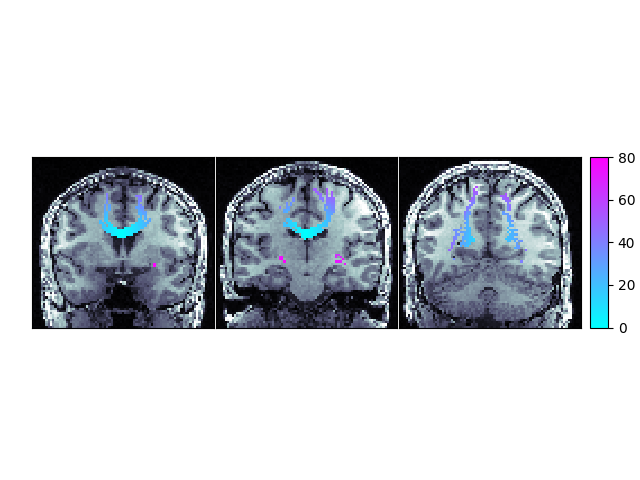
The next function we’ll demonstrate is density_map. This function allows one to represent the spatial distribution of a track by counting the density of streamlines in each voxel. For example, let’s take the track connecting the left and right superior frontal gyrus.

lr_superiorfrontal_track = grouping[11, 54]
shape = labels.shape
dm = utils.density_map(lr_superiorfrontal_track, affine, shape)

Let’s save this density map and the streamlines so that they can be visualized together. In order to save the streamlines in a “.trk” file we’ll need to move them to “trackvis space”, or the representation of streamlines specified by the trackvis Track File format.

# Save density map
save_nifti("lr-superiorfrontal-dm.nii.gz", dm.astype("int16"), affine)

lr_sf_trk = Streamlines(lr_superiorfrontal_track)

# Save streamlines
sft = StatefulTractogram(lr_sf_trk, hardi_img, Space.VOX)
save_trk(sft, "lr-superiorfrontal.trk")

Footnotes

[1]

The image aparc-reduced.nii.gz, which we load as labels_img, is a modified version of label map aparc+aseg.mgz created by FreeSurfer. The corpus callosum region is a combination of the FreeSurfer labels 251-255. The remaining FreeSurfer labels were re-mapped and reduced so that they lie between 0 and 88. To see the FreeSurfer region, label and name, represented by each value, see label_info.txt in ~/.dipy/stanford_hardi.

[2]

An affine transformation is a mapping between two coordinate systems that can represent scaling, rotation, shear, translation and reflection. Affine transformations are often represented using a 4x4 matrix where the last row of the matrix is [0, 0, 0, 1].