Signal Reconstruction Using Spherical Harmonics

This example shows how you can use a spherical harmonics (SH) function to reconstruct any spherical function using DIPY. In order to generate a signal, we will need to generate an evenly distributed sphere.

Let’s import some standard packages.

import numpy as np

from dipy.core.sphere import HemiSphere, Sphere, disperse_charges
from dipy.data import get_sphere
from dipy.reconst.shm import sf_to_sh, sh_to_sf
from dipy.sims.voxel import multi_tensor_odf
from dipy.viz import actor, window

We can first create some random points on a HemiSphere using spherical polar coordinates.

rng = np.random.default_rng()
n_pts = 64
theta = np.pi * rng.random(n_pts)
phi = 2 * np.pi * rng.random(n_pts)
hsph_initial = HemiSphere(theta=theta, phi=phi)

Next, we call disperse_charges which will iteratively move the points so that the electrostatic potential energy is minimized. In hsph_updated we have the updated HemiSphere with the points nicely distributed on the hemisphere.

hsph_updated, potential = disperse_charges(hsph_initial, 5000)
sphere = Sphere(xyz=np.vstack((hsph_updated.vertices, -hsph_updated.vertices)))

We now need to create our initial signal. To do so, we will use our sphere’s vertices as the sampled points of our spherical function (SF). We will use multi_tensor_odf to simulate an ODF. For more information on how to use DIPY to simulate a signal and ODF, see MultiTensor Simulation.

mevals = np.array([[0.0015, 0.00015, 0.00015], [0.0015, 0.00015, 0.00015]])
angles = [(0, 0), (60, 0)]
odf = multi_tensor_odf(sphere.vertices, mevals, angles, [50, 50])

# Enables/disables interactive visualization
interactive = False

scene = window.Scene()
scene.SetBackground(1, 1, 1)

odf_actor = actor.odf_slicer(odf[None, None, None, :], sphere=sphere)
odf_actor.RotateX(90)
scene.add(odf_actor)

print("Saving illustration as symm_signal.png")
window.record(scene=scene, out_path="symm_signal.png", size=(300, 300))
if interactive:
    window.show(scene)

Saving illustration as symm_signal.png

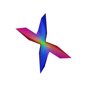
Illustration of the simulated signal sampled on a sphere of 64 points per hemisphere

We can now express this signal as a series of SH coefficients using sf_to_sh. This function converts a series of SF coefficients in a series of SH coefficients. For more information on SH basis, see Spherical Harmonic bases. For this example, we will use the descoteaux07 basis up to a maximum SH order of 8.

# Change this value to try out other bases
sh_basis = "descoteaux07"
# Change this value to try other maximum orders
sh_order_max = 8

sh_coeffs = sf_to_sh(odf, sphere, sh_order_max=sh_order_max, basis_type=sh_basis)

sh_coeffs is an array containing the SH coefficients multiplying the SH functions of the chosen basis. We can use it as input of sh_to_sf to reconstruct our original signal. We will now reproject our signal on a high resolution sphere using sh_to_sf.

high_res_sph = get_sphere(name="symmetric724").subdivide(n=2)
reconst = sh_to_sf(
    sh_coeffs, high_res_sph, sh_order_max=sh_order_max, basis_type=sh_basis
)

scene.clear()
odf_actor = actor.odf_slicer(reconst[None, None, None, :], sphere=high_res_sph)
odf_actor.RotateX(90)
scene.add(odf_actor)

print("Saving output as symm_reconst.png")
window.record(scene=scene, out_path="symm_reconst.png", size=(300, 300))
if interactive:
    window.show(scene)

Saving output as symm_reconst.png

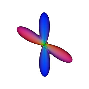
Reconstruction of a symmetric signal on a high resolution sphere using a symmetric basis

While a symmetric SH basis works well for reconstructing symmetric SF, it fails to do so on asymmetric signals. We will now create such a signal by using a different ODF for each hemisphere of our sphere.

mevals = np.array([[0.0015, 0.0003, 0.0003]])
angles = [(0, 0)]
odf2 = multi_tensor_odf(sphere.vertices, mevals, angles, [100])

n_pts_hemisphere = int(sphere.vertices.shape[0] / 2)
asym_odf = np.append(odf[:n_pts_hemisphere], odf2[n_pts_hemisphere:])

scene.clear()
odf_actor = actor.odf_slicer(asym_odf[None, None, None, :], sphere=sphere)
odf_actor.RotateX(90)
scene.add(odf_actor)

print("Saving output as asym_signal.png")
window.record(scene=scene, out_path="asym_signal.png", size=(300, 300))
if interactive:
    window.show(scene)

Saving output as asym_signal.png

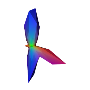
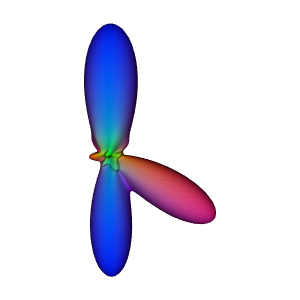
Illustration of an asymmetric signal sampled on a sphere of 64 points per hemisphere

Let’s try to reconstruct this SF using a symmetric SH basis.

sh_coeffs = sf_to_sh(asym_odf, sphere, sh_order_max=sh_order_max, basis_type=sh_basis)
reconst = sh_to_sf(
    sh_coeffs, high_res_sph, sh_order_max=sh_order_max, basis_type=sh_basis
)

scene.clear()
odf_actor = actor.odf_slicer(reconst[None, None, None, :], sphere=high_res_sph)
odf_actor.RotateX(90)
scene.add(odf_actor)

print("Saving output as asym_reconst.png")
window.record(scene=scene, out_path="asym_reconst.png", size=(300, 300))
if interactive:
    window.show(scene)

Saving output as asym_reconst.png

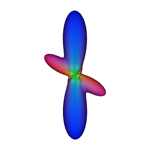
Reconstruction of an asymmetric signal using a symmetric SH basis

As we can see, a symmetric basis fails to properly represent asymmetric SF. Fortunately, DIPY also implements full SH bases, which can deal with symmetric as well as asymmetric signals. For this tutorial, we will demonstrate it using the descoteaux07 full SH basis by setting full_basis=true.

sh_coeffs = sf_to_sh(
    asym_odf, sphere, sh_order_max=sh_order_max, basis_type=sh_basis, full_basis=True
)
reconst = sh_to_sf(
    sh_coeffs,
    high_res_sph,
    sh_order_max=sh_order_max,
    basis_type=sh_basis,
    full_basis=True,
)

scene.clear()
odf_actor = actor.odf_slicer(reconst[None, None, None, :], sphere=high_res_sph)
odf_actor.RotateX(90)
scene.add(odf_actor)

print("Saving output as asym_reconst_full.png")
window.record(scene=scene, out_path="asym_reconst_full.png", size=(300, 300))
if interactive:
    window.show(scene)

Saving output as asym_reconst_full.png

Reconstruction of an asymmetric signal using a full SH basis

As we can see, a full SH basis properly reconstruct asymmetric signal.